Machine Learning from Human Preferences
Chapter 3: Elicitation
Overview
- Chapters 2–3 established models and learned their parameters
- Now: which queries should we ask?
- Human feedback is expensive — strategically chosen comparisons can save 80% of annotation cost
- Central tool: Fisher information + optimal experimental design
- Key insight: not all comparisons are equally informative
Chapter Roadmap
Lecture 1 — Preference Vectors & Metric Elicitation
- Fisher information & Rasch model (15 min)
- Factor models & D/A/E-optimal design (15 min)
- Pairwise preferences & Sherman-Morrison (10 min)
- Metric elicitation via binary search (10 min)
Lecture 2 — Preference Functions & Active DPO
- Linear & nonlinear preference functions (15 min)
- GP active learning (15 min)
- Active DPO for LLM alignment (15 min)
- Summary (5 min)
Connections to Prior Chapters
| Bradley-Terry model |
Fisher information, query selection |
| Factor models \(U^\top V\) |
D-optimal pair selection |
| GP preference models |
Information-gain acquisition |
| DPO loss |
ADPO active selection |
“The purpose of optimal design is to achieve the desired precision with minimum cost.” — V.V. Fedorov (1972)
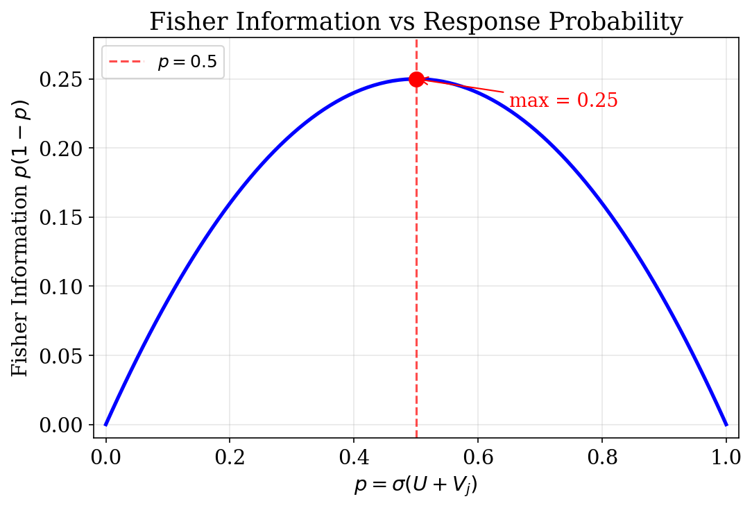
1. Fisher Info for the Rasch Model
For item \(j\) with \(p_j(U) = \sigma(U + V_j)\):
\[
\mathcal{I}_j(U) = p_j(U)(1 - p_j(U))
\]
![]()
1. Optimal Item Difficulty
Proposition. \(\mathcal{I}_j(U) = p_j(1 - p_j)\) is maximized when \(p_j = 0.5\), i.e., item difficulty \(-V_j\) equals user ability \(U\).
- Items that are too easy (\(p \approx 1\)): near-deterministic, teach little
- Items that are too hard (\(p \approx 0\)): also uninformative
- Items matched to ability (\(p \approx 0.5\)): maximally informative
- Best next item: difficulty \(-V_j\) close to current estimate of \(U\)
1. Active Item Selection
Score and cumulative information with prior \(U \sim \mathcal{N}(0, \sigma_0^2)\):
\[
\begin{aligned}
S(U) &= \sum_{j \in \mathcal{J}} (y_j - p_j(U)) \\
\mathcal{I}(U) &= \sum_{j \in \mathcal{J}} p_j(U)(1 - p_j(U)) + \tau_0
\end{aligned}
\]
- Newton update: \(\hat{U} \leftarrow \hat{U} + S(\hat{U}) / \mathcal{I}(\hat{U})\)
- Selection rule: \(j_t = \arg\max_j \; p_j(\hat{U})(1 - p_j(\hat{U}))\)
- Posterior variance: \(\widehat{\text{Var}}(U) \approx \mathcal{I}(\hat{U})^{-1}\)
- Reliability: \(\text{Rel} \approx 1 - \tfrac{1}{N}\sum_i \widehat{\text{Var}}(U_i) / \sigma_U^2\)
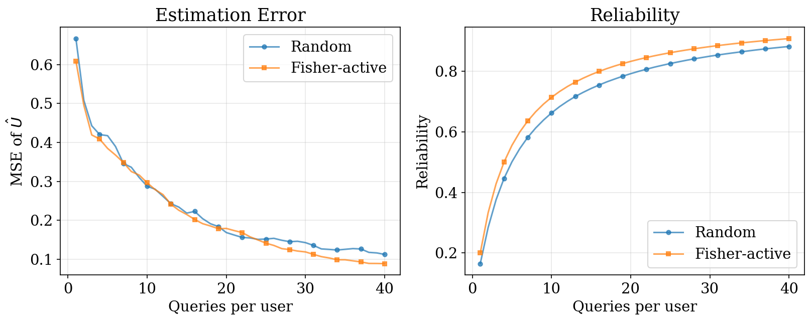
1. Fisher-Active vs Random
![]()
Fisher-active selection achieves higher reliability with fewer queries by targeting items near \(p = 0.5\).
1. Key Insight
Measure where uncertainty is highest.
- Items near \(p = 0.5\) are maximally informative
- Active selection “hovers” around the user’s current location
- This principle underlies all active learning methods in this chapter:
- Rasch \(\rightarrow\) Factor models \(\rightarrow\) Pairwise \(\rightarrow\) GPs \(\rightarrow\) DPO
2. Factor Models: Multi-Dimensional Preferences
Generalize Rasch to \(K\) dimensions: \(H_{ij} = U_i^\top V_j + Z_j\)
- User embedding \(U_i \in \mathbb{R}^K\), item embedding \(V_j \in \mathbb{R}^K\)
- Fisher information per item is a rank-1 matrix:
\[
\mathcal{I}_j(U) = \sigma(H)(1 - \sigma(H)) \; V_j V_j^\top
\]
- Cumulative: \(\mathcal{I}(U) = \sum_t \sigma(H_{j_t})(1 - \sigma(H_{j_t})) \; V_{j_t} V_{j_t}^\top\)
- Each item contributes information in the direction of \(V_j\)
2. Optimal Design Criteria (D/A/E)
Given Fisher information matrix \(\mathcal{I}(U)\):
| A-Optimal |
min tr(\(\mathcal{I}^{-1}\)) |
Average variance |
| D-Optimal |
max det(\(\mathcal{I}\)) |
Volume shrinkage of posterior ellipsoid |
| E-Optimal |
max \(\lambda_{\min}(\mathcal{I})\) |
Worst-case precision |
- All three reduce uncertainty, but emphasize different aspects
- D-optimal naturally encourages diversity — redundant directions give diminishing gain
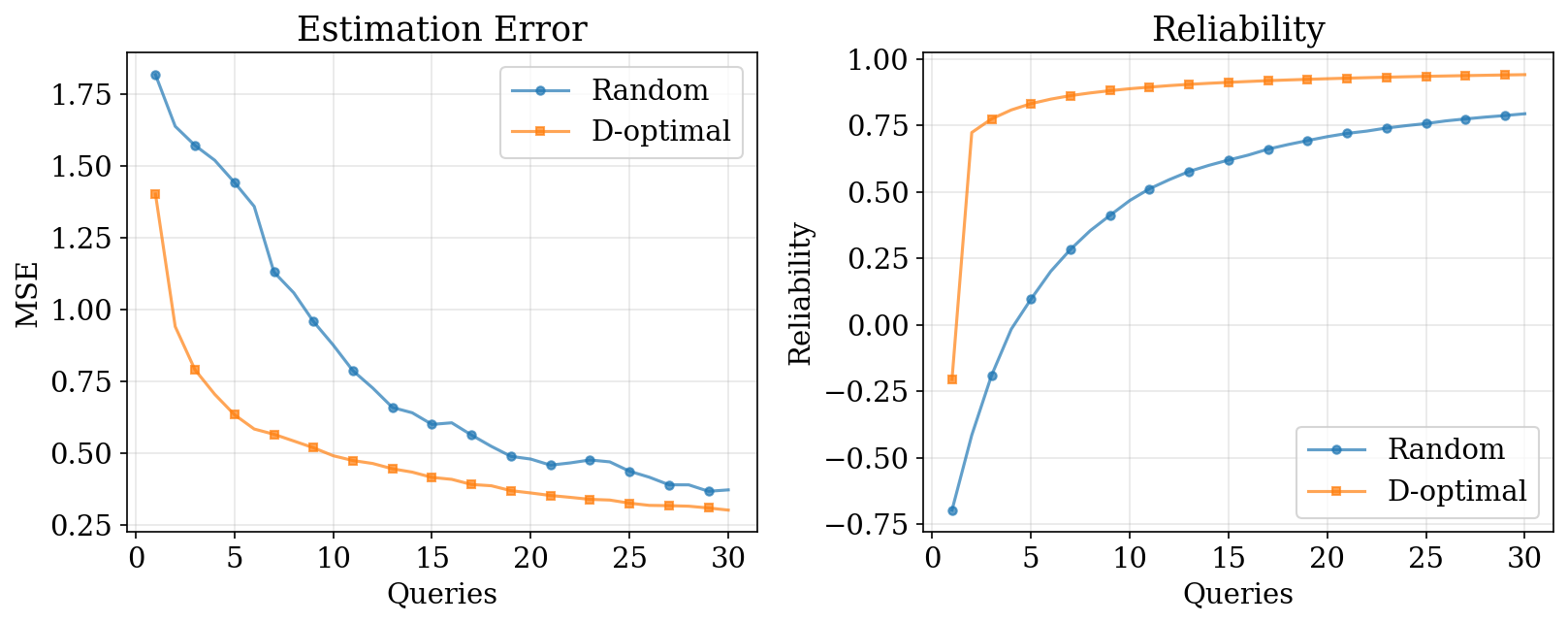
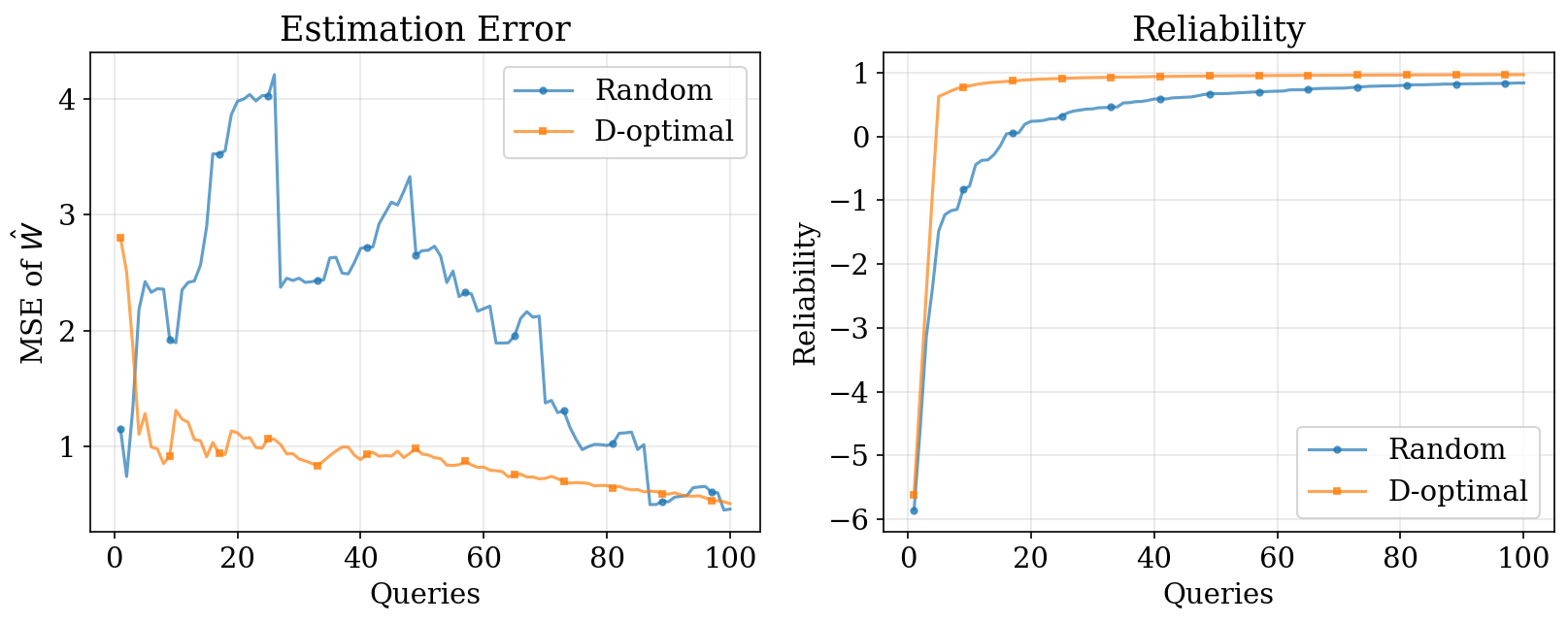
2. D-Optimal Selection for Factor Models
- Pick next item maximizing \(\det(\mathcal{I} + \mathcal{I}_j)\)
- Reliability generalized: \(\text{Rel} = 1 - \text{tr}(\hat{\Sigma}_{\text{err}}) / \text{tr}(\Sigma_U)\)
![]()
3. Pairwise Preferences
Bradley-Terry for pairs: \(p(j \succ k) = \sigma(U^\top(V_j - V_k) + Z_j - Z_k)\)
- Feature difference: \(x_{jk} = V_j - V_k\)
- Fisher information per pair:
\[
\mathcal{I}_{jk}(U) = w \cdot x_{jk} x_{jk}^\top, \quad w = p(1 - p)
\]
- Posterior precision accumulates additively:
\[
\Lambda_t = \Sigma_0^{-1} + \sum_{s \leq t} w_s \, x_s x_s^\top
\]
3. D-Optimal via Sherman-Morrison
Proposition. The D-optimal acquisition has closed form:
\[
\Delta_D(j,k) = \log\det(\Lambda + w\,xx^\top) - \log\det(\Lambda) = \log(1 + w \, x^\top \Sigma \, x)
\]
- Follows from the matrix determinant lemma: \(\det(A + uv^\top) = (1 + v^\top A^{-1} u)\det(A)\)
- Only requires a vector-matrix-vector product — efficient for online selection
- A-optimal: \(\Delta_A = \tfrac{w \, x^\top \Sigma^2 x}{1 + w \, x^\top \Sigma \, x}\)
- E-optimal proxy: \(\Delta_E^{\text{proxy}} = w \, x^\top \Sigma \, x\)
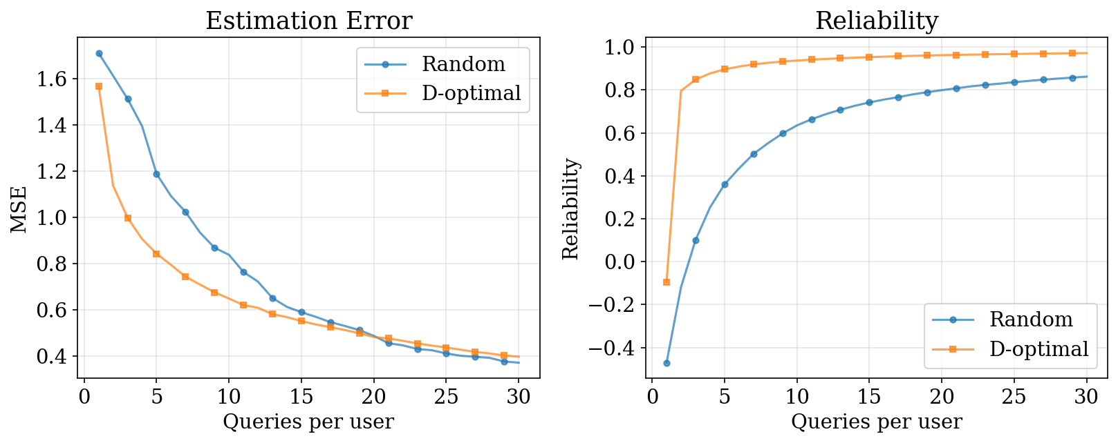
3. Pairwise D-Optimal: Results
![]()
D-optimal selection shrinks the posterior ellipsoid efficiently in all directions.
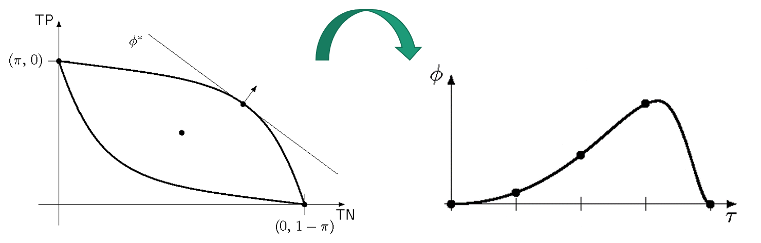
4. Metric Elicitation: Motivation
- Different classifiers trade off error types differently
- Which is “best” depends on the implicit metric
- Medical diagnosis: false negatives (missed disease) are costly
- Spam filtering: false positives (lost email) are costly
- The practitioner’s metric \(\mathbf{m}^*\) is unknown
4. Metric Elicitation as Factor Model
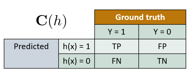
Metric elicitation is a \(K=2\) factor model with known item parameters:
- “Items” = classifiers with known confusion matrices \(V_\theta = (\text{TP}_\theta, \text{TN}_\theta)\)
- “User preference” = unknown metric weights \(\mathbf{m} = (m_{11}, m_{00})\)
- Linear Performance Metric: \(\phi(C) = m_{11} \cdot \text{TP} + m_{00} \cdot \text{TN} + m_0\)
- Parametrize: \(\mathbf{m} = (\cos\theta, \sin\theta)\) for \(\theta \in [0, 2\pi]\)
![]()
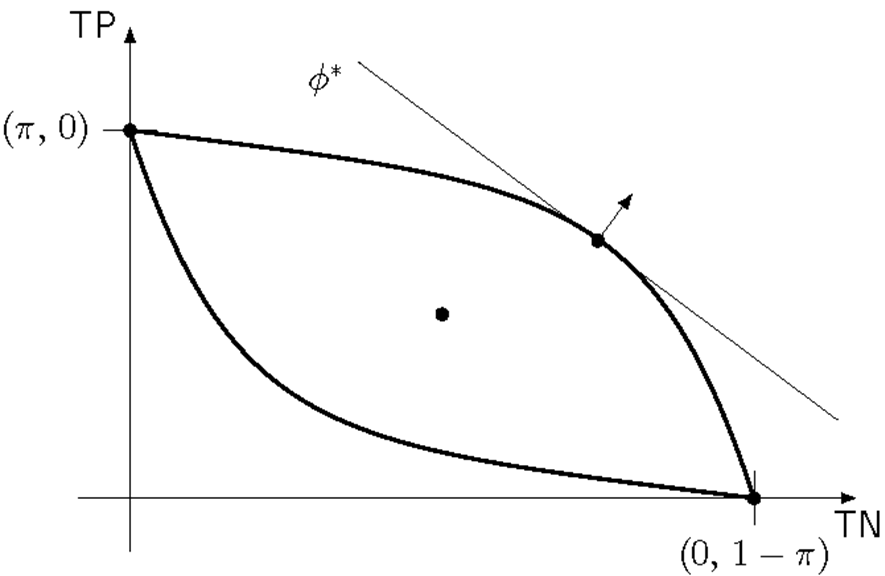
4. Quasiconcavity & Binary Search
Proposition. For a quasiconcave LPM, the composition \(\phi \circ \rho^+\) with the upper boundary of the confusion matrix space is unimodal.
![]()
- Unimodality \(\Rightarrow\) no local maxima \(\Rightarrow\) binary search works
- Each iteration: 4 queries, shrinks interval by factor 2
4. Binary Search Algorithm
![]()
- Query complexity: \(O(\log(1/\epsilon))\) — exponentially better than general 2D estimation at \(O(1/\epsilon^2)\)
- Works even under noise with probabilistic oracle responses
4. Metric Elicitation: Extensions
- Bayes optimal classifier: \(\bar{h}(x) = \mathbf{1}[\eta(x) \geq m_{00}/(m_{11} + m_{00})]\)
- Learning the metric = learning the optimal classification threshold
- Linear-fractional metrics (\(F_\beta\), Jaccard): two binary searches, still \(O(\log(1/\epsilon))\)
- Multiclass: diagonal LPMs with \(K\) classes \(\Rightarrow\) \(O(K^2 \log(1/\epsilon))\) queries
5. Linear Preference Functions
Items scored by shared weight vector: \(V_j = W^\top X_j\)
\[
p(j \succ k) = \sigma(W^\top(X_j - X_k))
\]
- This is logistic regression on pairwise feature differences \(x_{jk} = X_j - X_k\)
- Fisher information: \(\mathcal{I}(W) = p(1-p) \, x_{jk} x_{jk}^\top\)
- Laplace posterior: \(\Sigma \approx (\sigma_0^{-2}I + \sum_t p_t(1-p_t) \, x_t x_t^\top)^{-1}\)
- Same D-optimal criterion: \(\Delta_D(j,k) = \log(1 + w \, x^\top \Sigma \, x)\)
5. Linear Preference: Results
![]()
D-optimal selection converges faster with the same mathematical framework as before.
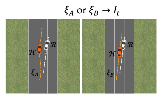
5. Robotic Trajectory Learning
Trajectory reward: \(R(\xi) = w^\top \phi(\xi)\)
- Unknown weights \(w\), known features \(\phi(\xi)\)
- Each comparison “prefer \(\xi_A\) over \(\xi_B\)” gives a half-space constraint: \(w^\top(\phi(\xi_A) - \phi(\xi_B)) \succ 0\)
- Acquisition: maximize minimum volume removed regardless of answer
Biyik and Sadigh (2018)
5. Trajectory Learning: Results & Extensions
- Driving simulator: 0 queries \(\rightarrow\) erratic; 30 queries \(\rightarrow\) lane following; 70 queries \(\rightarrow\) collision avoidance
- Active selection achieves target performance faster — critical for time-sensitive applications (e.g., exoskeleton rehabilitation)
- Foundation models (R3M, Voltron): pretrained representations give 2–3x higher success with 5–10x fewer demos
5. Non-Linear Scoring Functions
For non-linear scorer \(V_j = f_\theta(X_j)\), linearize around \(\hat\theta\):
\[
f_\theta(X_j) \approx f_{\hat\theta}(X_j) + J_j \,\Delta\theta, \quad J_j = \left.\frac{\partial f_\theta(X_j)}{\partial \theta}\right|_{\hat\theta}
\]
Pairwise logit:
\[
\underbrace{f_\theta(X_j) - f_\theta(X_k)}_{\text{logit}} \approx \underbrace{f_{\hat\theta}(X_j) - f_{\hat\theta}(X_k)}_{\text{offset}} + \underbrace{(J_j - J_k)}_{\phi_{jk}} \Delta\theta
\]
5. D-Optimal for Nonlinear Models
Replace \(x_{jk}\) with Jacobian difference \(\phi_{jk} = J_j - J_k\):
\[
\Sigma^{-1} = \sigma_0^{-2}I + \sum_t w_t \, \phi_t^\top \phi_t
\]
- D-optimal: \(\Delta_D(j,k) = \log(1 + w \, \phi \, \Sigma \, \phi^\top)\)
- A-optimal: \(\Delta_A(j,k) = \tfrac{w \, \phi \, \Sigma^2 \, \phi^\top}{1 + w \, \phi \, \Sigma \, \phi^\top}\)
- Only needs Jacobian rows + vector-matrix-vector product
- Same structure as linear case — local linearization is the key trick
6. GP Active Learning: Motivation
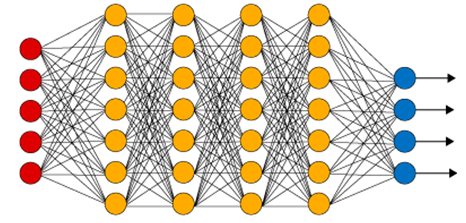
- Previous sections: parametric models (Rasch, linear, neural net)
- Gaussian Processes: nonparametric, flexible, natural uncertainty
- GP posterior variance varies across input space
- Key question: how to actively select queries for GP preference models?
- Insight: GP uncertainty naturally guides query selection
6. Practical Computation
Using Laplace approximation:
\[
a(x_A, x_B) = h\!\left(\Phi\!\left(\frac{\mu_A - \mu_B}{\sqrt{2\sigma_{\text{noise}}^2 + g(x_A, x_B)}}\right)\right) - m(x_A, x_B)
\]
where \(g(x_A, x_B) = \sigma_A^2 + \sigma_B^2 - 2\text{Cov}(r(x_A), r(x_B))\)
- \(h(p)\): binary entropy; \(\Phi\): normal CDF
- Key property: trivial query \((x, x)\) is a global minimizer — avoids degenerate queries
6. GP Active Learning Algorithm
- Initialize GP prior over reward function
- For each round \(t = 1, \ldots, T\):
- Compute acquisition \(a(x_A, x_B)\) for all candidate pairs
- Select pair \((x_A^*, x_B^*)\) maximizing acquisition
- Query oracle for preference
- Update GP posterior via Laplace approximation
- Return learned reward function with uncertainty
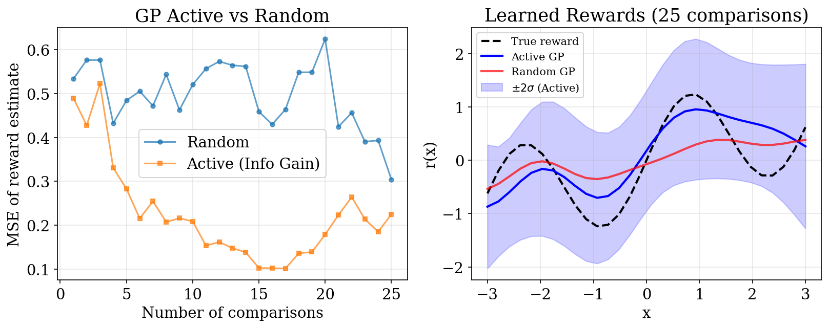
6. GP Active Learning: Results
![]()
Active selection targets uncertain regions, achieving lower error with fewer comparisons.
6. When to Use GP Active Learning
| Nonlinear reward structure |
GP strongly preferred |
| Low-to-moderate dimensions (\(d \lesssim 10\)) |
GP works well |
| Expensive human feedback |
Active learning essential |
| Need uncertainty quantification |
GP provides naturally |
| Large datasets (\(n \succ 1000\)) |
Consider sparse GP |
| Very high dimensions |
Linear models more practical |
7. Active DPO: Motivation
Recall DPO assumes Bradley-Terry preferences:
\[
p(y_w \succ y_l \mid x) = \sigma\!\left(\beta \log \frac{\pi_\theta(y_w \mid x)}{\pi_{\text{ref}}(y_w \mid x)} - \beta \log \frac{\pi_\theta(y_l \mid x)}{\pi_{\text{ref}}(y_l \mid x)}\right)
\]
- LLMs have billions of parameters — exact Fisher information is intractable
- How can we apply D-optimal design principles from Sections 1–5?
7. Log-Linear Policy Assumption
Approximate policy as log-linear in last-layer features:
\[
\pi(y \mid x; \theta) \propto \exp(\phi(x, y)^\top \theta)
\]
- Justified by neural tangent kernel perspective
- DPO loss Hessian takes the form:
\[
H(\theta) = \sum_{i=1}^n p_i(1 - p_i) \cdot \Delta\phi_i \, \Delta\phi_i^\top
\]
where \(\Delta\phi_i = \phi(x_i, y_{w,i}) - \phi(x_i, y_{l,i})\)
This IS the Fisher information matrix!
7. DPO D-Optimal Criterion
D-optimal selection for DPO:
\[
\max_S \; \log\det\!\left(\sum_{i \in S} p_i(1 - p_i) \cdot \Delta\phi_i \, \Delta\phi_i^\top\right)
\]
- Same mathematical structure as all previous sections
- Feature difference: \(\Delta\phi_i = \phi(x_i, y_{w,i}) - \phi(x_i, y_{l,i})\)
- Sherman-Morrison still applies for sequential selection
7. ADPO Algorithm
Active DPO (ADPO):
- Compute features: \(\Delta\phi_i = \phi(x_i, y_{i,1}) - \phi(x_i, y_{i,2})\)
- D-optimal selection: \[
i^* = \arg\max_i \; \log\det\!\left(I + p_i(1 - p_i) \, H_t^{-1} \Delta\phi_i \, \Delta\phi_i^\top\right)
\]
- Query oracle: obtain human preference for pair \(i^*\)
- Update: add to training set, retrain with DPO loss
7. ADPO Convergence
Theorem. Under log-linear policy + regularity conditions:
\[
\|\hat\theta_n - \theta^*\| = O\!\left(\frac{d}{\sqrt{n}}\right)
\]
- Matches the minimax optimal rate for \(d\)-dimensional estimation
- D-optimal ensures Fisher information grows proportionally to \(n\)
- Key: effective dimension \(d\) is the rank of the Fisher information matrix (last-layer features), not the full parameter count
7. ADPO+ for Offline Settings
- Pool-based: select from existing unlabeled pairs (fixed response pool)
- Batch selection: select \(b\) queries at once for parallel annotation
- Diversity: D-optimal naturally encourages diversity — redundant queries give diminishing log-det gain
- Practical for production RLHF pipelines with fixed candidate pairs
7. When Does Active Learning Help for DPO?
| Annotation cost |
High cost \(\rightarrow\) essential |
| Data heterogeneity |
Diverse prompts \(\rightarrow\) more room for selection |
| Budget constraints |
Limited budget (\(\lt\) 10K) \(\rightarrow\) largest gains |
| Model capacity |
Larger models \(\rightarrow\) helps reduce overfitting |
| Query pool size |
Large pool \(\rightarrow\) more room for intelligent selection |
7. GP Active Learning vs ADPO
| Model |
Nonparametric (GP) |
Parametric (neural) |
| Scalability |
\(O(n^3)\) |
\(O(d^2 n)\) |
| Use case |
Small datasets, uncertainty |
LLM alignment, large models |
| Acquisition |
Information gain |
D-optimal design |
| Theory |
Mutual information |
Fisher information |
Both share the core insight: use model uncertainty to guide query selection.
Summary: Key Equations
- D-optimal (Sherman-Morrison): \(\Delta_D = \log(1 + w \, x^\top \Sigma \, x)\)
- Metric elicitation: \(O(\log(1/\epsilon))\) queries via binary search on unimodal boundary
- ADPO convergence: \(\|\hat\theta_n - \theta^*\| = O(d / \sqrt{n})\)
All use the same principle: measure where uncertainty is highest, whether that’s item difficulty, posterior covariance, or GP predictive variance.
Practical Guidance
| Scalar ability (testing, psychometrics) |
Rasch + Fisher active |
| Multi-dimensional preferences |
Factor model + D-optimal |
| Known item features |
Linear preference + D-optimal |
| Unknown nonlinear reward |
GP active learning |
| LLM alignment |
ADPO |
| Metric design |
Binary search on LPM |