Machine Learning from Human Preferences

Chapter 2: Learning

Overview

Chapter 2 established models (Rasch, Bradley-Terry, factor models); now we learn their parameters
Four complementary approaches:
1. Maximum Likelihood Estimation — fast, scalable, point estimates
2. Bayesian Inference — uncertainty quantification via MCMC and GPs
3. Online Learning — incremental updates for streaming data (Elo)
4. Practical ML — regularization, cross-validation, modern optimizers

Chapter Roadmap

Lecture 1: Core parameter estimation

Maximum likelihood estimation for Bradley-Terry (20 min)
Bayesian inference: MCMC and Gaussian Processes (20 min)
Comparison of methods (10 min)

Lecture 2: Advanced learning topics

Online learning with Elo ratings (15 min)
Regularization and overfitting (15 min)
Cross-validation and model selection (10 min)
Optimization: Adam, learning rate schedules (10 min)

Maximum Likelihood Estimation

Given observed preference data, find parameters that maximize the probability of the data
MLE is the most common approach: fast, scalable, well-understood
Provides point estimates only — no uncertainty quantification
Steps: train/test split $\rightarrow$ define objective $\rightarrow$ derive gradient $\rightarrow$ optimize

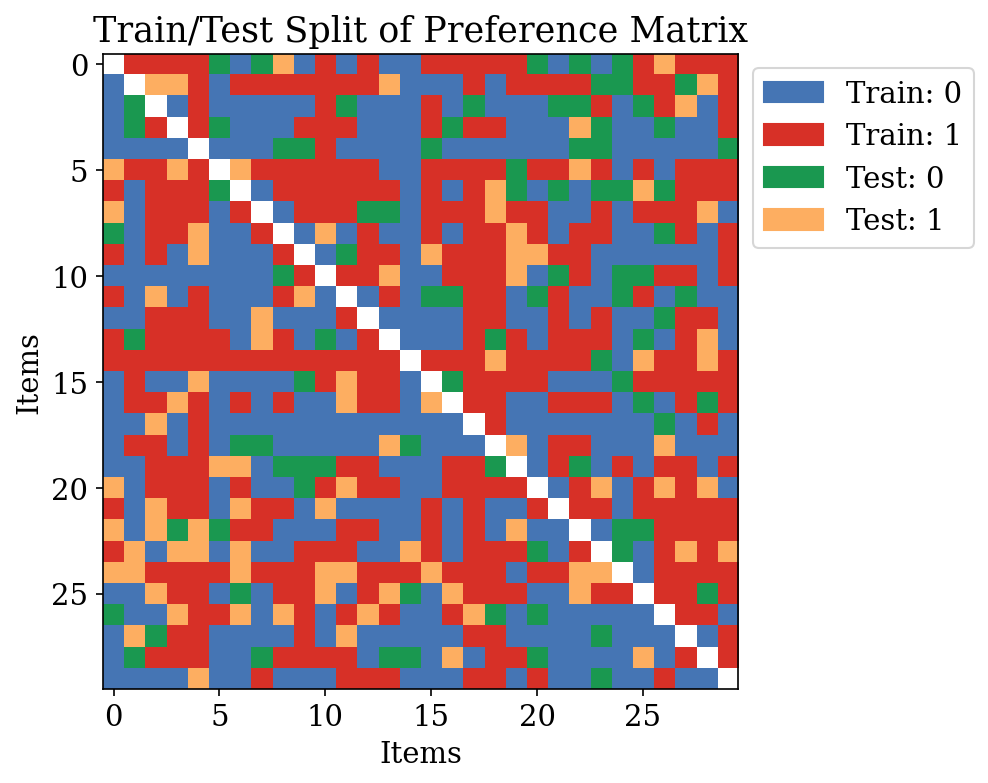
Train/Test Split for Preference Data

Randomly partition observed pairwise comparisons: 80% train / 20% test
For preference data: partition comparisons (not items) into splits
Each entry: $Y_{jj'} \in \{0, 1\}$ — whether item $j$ beats item $j'$

MLE Objective

For Bradley-Terry with items $j \in \{1, \ldots, M\}$:

\[ \hat{V} = \arg\max_{V} \sum_{(j,j') \in \mathcal{D}_{\text{train}}} \log p(Y_{jj'} \mid \sigma(V_j - V_{j'})) \]

Log-likelihood is concave when the comparison graph is connected
Optimize with gradient descent
Each item has a single scalar parameter $V_j$ (its “strength” or “utility”)

MLE Gradient

Define residuals: $r_{mk} = y_{mk} - \sigma(V_m - V_k)$ (observed $-$ predicted)

\[ \frac{\partial \ell}{\partial V_m} = \sum_{(m,k)\in \mathcal{N}^+_m} r_{mk} - \sum_{(k,m)\in \mathcal{N}^-_m} r_{km} \]

$\mathcal{N}^+_m$: pairs where $m$ is listed first; $\mathcal{N}^-_m$: pairs where $m$ is listed second
If $m$ beats $k$ more than predicted: residual positive $\Rightarrow$ push $V_m$ up
If $m$ loses to $k$ more than predicted: residual negative $\Rightarrow$ push $V_m$ down

MLE Gradient: Intuition

Each comparison contributes a residual = observed $-$ predicted
Gradient is a sum of residuals across all opponents of item $m$
Surprise drives learning: unexpected outcomes cause large updates
Expected outcomes cause small updates (residual $\approx 0$)
This is equivalent to logistic regression on the differences $V_j - V_k$

MLE Training: AUC Convergence

Learned vs True Utilities

Bayes Optimal AUC

Even with perfect parameters, test AUC $\lt 1.0$ due to label noise
Bayes optimal: rank by true win probabilities $P_{jk} = \sigma(V_j - V_k)$
MLE achieves close to Bayes optimal when data is sufficient
Fundamental limit from stochastic nature of preference data

Bayesian Inference for Preferences

Alternative to MLE: place a prior on parameters, update with data to get posterior
Posterior distribution captures both central estimates and uncertainty
Two flavors:
- Parametric (MCMC): finite-dimensional $V$ with Gaussian prior
- Nonparametric (GP + Laplace): function-space prior over reward

Bayesian Posterior for Bradley-Terry

Prior: $p(V) = \prod_{j=1}^M \mathcal{N}(V_j \mid 0, 1)$
Likelihood: $p(\mathcal{D} \mid V) = \prod_{(j,j')} \sigma(V_j - V_{j'})^{Y_{jj'}} (1 - \sigma(V_j - V_{j'}))^{1 - Y_{jj'}}$
Posterior: $p(V \mid \mathcal{D}) \propto p(\mathcal{D} \mid V) \, p(V)$
Denominator (evidence) is intractable $\Rightarrow$ need MCMC to sample

Metropolis-Hastings Algorithm

General MH acceptance probability:

\[ \alpha = \min\left\{1, \frac{p(V' \mid \mathcal{D}) \cdot q(V^{(t)} \mid V')}{p(V^{(t)} \mid \mathcal{D}) \cdot q(V' \mid V^{(t)})}\right\} \]

Propose new state: $V' \sim q(\cdot \mid V^{(t)})$
Accept with probability $\alpha$; otherwise stay at $V^{(t)}$
Chain converges to posterior distribution

MH with Symmetric Proposal

With Gaussian proposal $q(V' \mid V^{(t)}) = \mathcal{N}(V^{(t)}, \tau^2 I)$, the proposal terms cancel:

\[ \alpha = \min\left\{1, \frac{p(\mathcal{D} \mid V') \cdot p(V')}{p(\mathcal{D} \mid V^{(t)}) \cdot p(V^{(t)})}\right\} \]

Single-coordinate random walk: propose one $V_j$ at a time
Center after each step (fix shift invariance)
Tuning: proposal scale $\tau$ controls acceptance rate (target $$30-50%)

MCMC Trace Plot and Posterior

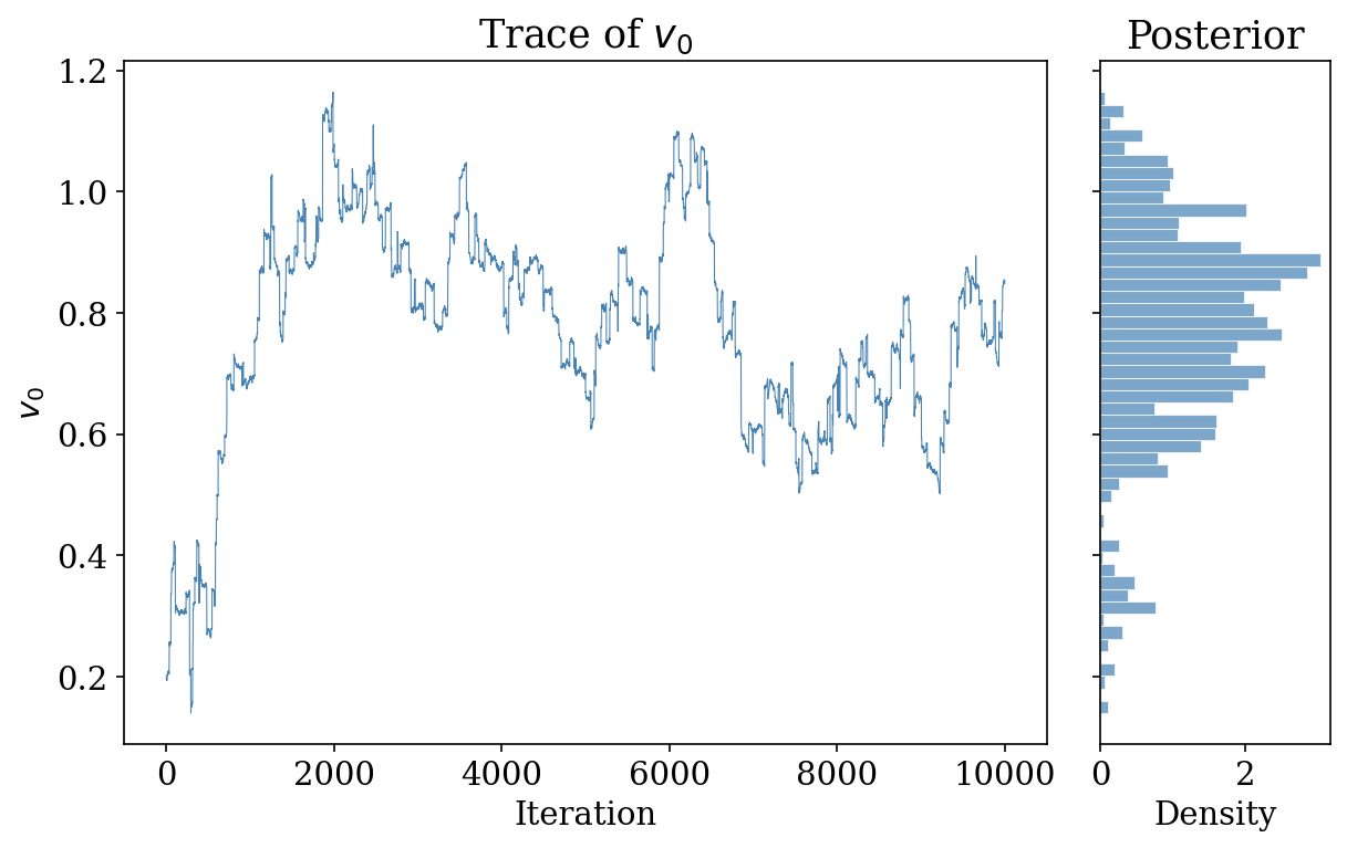
Left: trace of $v_0$ over MH iterations (good mixing)
Right: marginal posterior histogram for $v_0$
Posterior provides credible intervals for each item’s utility

Gaussian Processes for Preferences

What if the reward function is nonlinear and unknown?
GP prior: $r \sim \mathcal{GP}(m, k)$ over the reward function
Combine with Bradley-Terry likelihood: $p(y_i = 1 \mid r) = \sigma(r(x_A) - r(x_B))$
Sigmoid likelihood is non-Gaussian $\Rightarrow$ posterior is not a GP
Need approximation: Laplace approximation

Laplace Approximation

Find the posterior mode $\mathbf{r}^*$:

\[ \mathbf{r}^* = \arg\max_{\mathbf{r}} \sum_{i=1}^n \log \sigma\bigl(y_i(r(x_A^{(i)}) - r(x_B^{(i)}))\bigr) - \tfrac{1}{2}\mathbf{r}^\top K^{-1}\mathbf{r} \]

Approximate posterior as Gaussian centered at the mode
Uses Hessian of log-posterior as precision matrix

GP Gradient and Hessian

Gradient: $\nabla \log p(\mathbf{r} \mid \mathcal{D}) = \mathbf{g} - K^{-1}\mathbf{r}$

Hessian: $\nabla^2 \log p(\mathbf{r} \mid \mathcal{D}) = -W - K^{-1}$

where $W = \text{diag}(p_i(1-p_i))$ captures data-dependent precision

Newton’s method iteratively finds the mode: $\mathbf{r} \leftarrow \mathbf{r} - H^{-1} \nabla$
Each iteration is $O(m^3)$ where $m$ = number of unique points

Laplace Approximate Posterior

After finding $\mathbf{r}^*$:

\[ p(\mathbf{r} \mid \mathcal{D}) \approx \mathcal{N}\left(\mathbf{r}^*, (K^{-1} + W)^{-1}\right) \]

Structurally similar to GP regression, but with data-dependent precision $W$
$W$ arises from Bradley-Terry likelihood (not observation noise)
Enables posterior predictions with confidence intervals

GP Posterior with Confidence Intervals

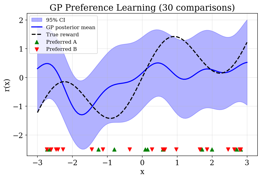
GP recovers nonlinear reward from pairwise comparisons
Uncertainty is wider where data is sparse
True reward (dashed) lies within the 95% confidence band

Fisher Information Connection

Observed Fisher information from Laplace: $I_{\text{obs}} = W = \text{diag}(p_i(1-p_i))$
Comparisons with $p \approx 0.5$ (uncertain outcomes) contribute most information
“Easy” comparisons (clear winner, $p \approx 0$ or $1$) contribute little
Connects to active learning (Chapter 4): query the most informative pairs

Online Learning: Motivation

Many settings: comparisons arrive sequentially (chess, online games, LLM evaluations)
Refitting full MLE after each observation is expensive
Need an incremental update rule: adjust only the two items involved
This is precisely the Elo rating system

Elo as Stochastic Gradient Ascent

SGD gradient of BT log-likelihood for a single comparison $(j, j')$:

\[ \frac{\partial \ell}{\partial V_j} = (y - p), \qquad \frac{\partial \ell}{\partial V_{j'}} = -(y - p) \]

Update with learning rate $\eta$ (the K-factor):

\[ V_j \leftarrow V_j + \eta(y - p), \qquad V_{j'} \leftarrow V_{j'} - \eta(y - p) \]

Elo Update: Intuition

If $j$ wins ($y=1$) but model predicted low $p$: large positive update to $V_j$
If $j$ wins but model predicted high $p$: small update (expected outcome)
If $j$ loses ($y=0$): opposite direction
Update magnitude $\propto$ surprise $|y - p|$

Elo = online learning algorithm for Bradley-Terry, interpretable as SGD with fixed step size

Elo Properties

K-factor ($\eta$): controls learning rate
- Large K: fast adaptation, noisy estimates
- Small K: stable estimates, slow adaptation
Zero-sum updates: total rating pool is conserved
Applications: chess (FIDE), online gaming (TrueSkill), LLM evaluation (Chatbot Arena)
Converges to MLE with decreasing step size (Robbins-Monro conditions)

MLE vs Bayesian vs Online

	MLE	Bayesian (MCMC)	Online (Elo)
Output	Point estimate	Posterior distribution	Point estimate
Uncertainty	No	Yes	No
Data	Batch	Batch	Sequential
Compute	Moderate	Expensive	Cheap per update
Best for	Large static datasets	Small data, uncertainty	Streaming data

All three methods estimate the same underlying Bradley-Terry parameters

Regularization: Why?

MLE maximizes training fit — can overfit with limited data
Overfitting: learned utilities capture noise, not true strengths
Symptoms: high training AUC, low test AUC
Regularization penalizes model complexity to improve generalization

L2 Regularization

Add a penalty to the log-likelihood:

\[ \mathcal{L}_{\text{reg}}(V) = \sum_{(j,j')} \log p(Y_{jj'} \mid V_j - V_{j'}) - \frac{\lambda}{2}\|V\|_2^2 \]

$\lambda = 0$: standard MLE
$\lambda \to \infty$: all utilities shrink to zero
$\lambda$ controls the bias-variance tradeoff

Regularized Gradient

\[ \frac{\partial \mathcal{L}_{\text{reg}}}{\partial V_m} = \sum_{(m,k)\in \mathcal{N}^+_m} r_{mk} - \sum_{(k,m)\in \mathcal{N}^-_m} r_{km} - \lambda V_m \]

Connection to Bayesian inference:

L2 regularization $=$ MAP estimation with Gaussian prior $\mathcal{N}(0, 1/\lambda)$

$\lambda$ is the inverse prior variance: large $\lambda$ $\Rightarrow$ tight prior near zero

Bias-Variance Tradeoff

Small $\lambda$: low bias, high variance (complex model, may overfit)
Large $\lambda$: high bias, low variance (simple model, may underfit)
Optimal $\lambda$: minimizes test error — balances both
Most critical when few observations relative to parameters

Validation Curve

Early Stopping

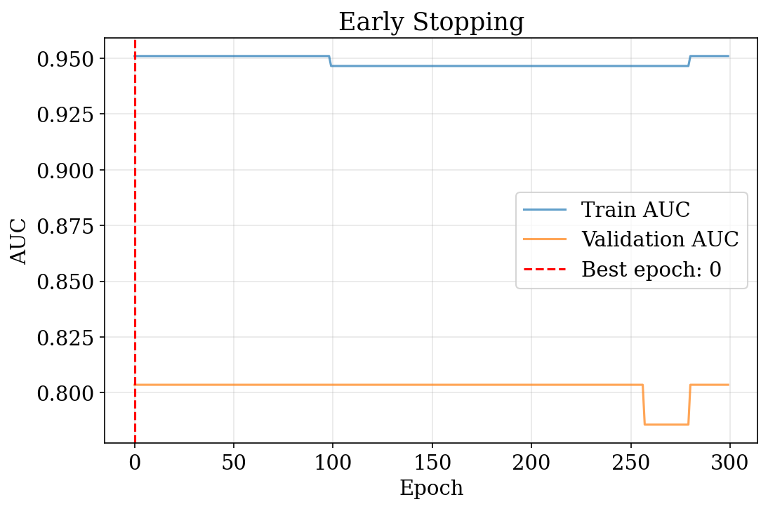
Alternative to explicit regularization: stop when validation performance peaks
GD follows a path from simple to complex models
No hyperparameter $\lambda$ to tune, but requires validation data

Model Selection: Motivation

A single train/test split has high variance: different splits give different results
We might over-tune to one particular split
Cross-validation systematically evaluates multiple splits
Enables principled hyperparameter selection and model comparison

K-Fold Cross-Validation

Partition data into $k$ equally-sized folds
For each fold $i$: train on all except fold $i$, evaluate on fold $i$
CV score: $\text{CV}_k = \frac{1}{k}\sum_{i=1}^k \text{metric}_i$

For preference data: partition comparisons (not items) into folds

Typically $k = 5$ or $k = 10$
Standard error quantifies uncertainty in the estimate

Hyperparameter Tuning with CV

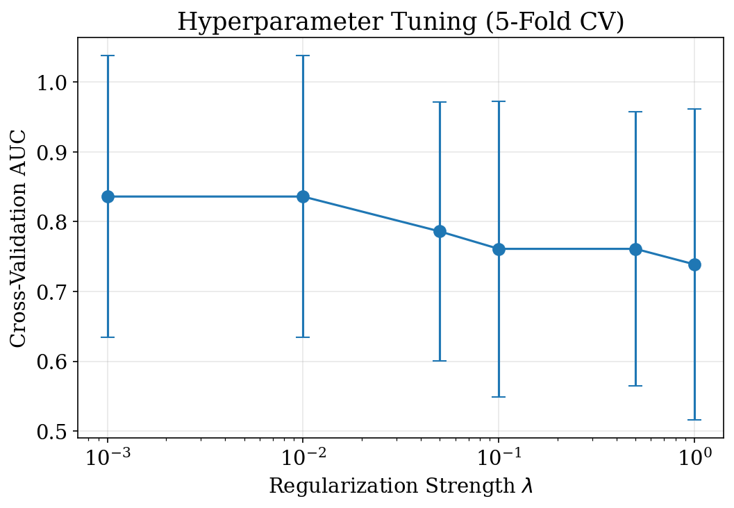
Grid search over $\lambda$ values using 5-fold CV
Select $\lambda$ with highest mean CV AUC
Error bars show standard deviation across folds

Evaluation Metrics: AUC

Area Under ROC Curve (AUC)

Measures ranking quality: probability that model correctly orders a random pair
For scores $s$ and labels $y$:

\[ \text{AUC} = \frac{\sum_{i: y_i=1} \sum_{j: y_j=0} \mathbf{1}[s_i \succ s_j]}{\sum_{i: y_i=1} \sum_{j: y_j=0} 1} \]

AUC $= 1.0$: perfect ranking; AUC $= 0.5$: random guessing
Does not capture calibration (probability accuracy)

Evaluation Metrics: Log-Likelihood and Calibration

Log-Likelihood

\[ \begin{aligned} \text{LL} = \sum &Y_{jj'}\log\sigma(V_j - V_{j'}) \\ +\, &(1\!-\!Y_{jj'})\log(1\!-\!\sigma(V_j\!-\!V_{j'})) \end{aligned} \]

Measures probability assigned to observed outcomes; higher is better

Calibration Error

Bin predictions into intervals
Compare average prediction to observed frequency
$\text{ECE} = \sum_b \frac{|B_b|}{N}|\bar{p}_b - \bar{y}_b|$
Perfect calibration: $\bar{p}_b = \bar{y}_b$ in each bin

Multi-Metric Comparison

AUC: ranking quality — does the model order items correctly?
Log-likelihood: probability quality — are predicted probabilities accurate?
Calibration: frequency matching — do predicted 70% events occur 70% of the time?

Different metrics may favor different models — use multiple for comprehensive evaluation

Beyond Vanilla Gradient Descent

Standard GD: $V \leftarrow V + \eta \nabla \mathcal{L}(V)$

Two limitations:

Fixed step size: large $\eta$ causes instability; small $\eta$ slows convergence
No momentum: each step ignores the optimization history

Modern optimizers address these through adaptive learning rates and momentum

Adam Optimizer

Adam (Adaptive Moment Estimation):

\[ \begin{aligned} m_t &\leftarrow \beta_1 m_{t-1} + (1-\beta_1)g_t \\ v_t &\leftarrow \beta_2 v_{t-1} + (1-\beta_2)g_t^2 \\ \hat{m}_t &\leftarrow m_t/(1-\beta_1^t), \quad \hat{v}_t \leftarrow v_t/(1-\beta_2^t) \\ V &\leftarrow V + \alpha\,\hat{m}_t / (\sqrt{\hat{v}_t}+\epsilon) \end{aligned} \]

Adam: Intuition

$m_t$: exponential moving average of gradients (momentum)
$v_t$: exponential moving average of squared gradients (variance)
Bias correction accounts for zero initialization in early iterations
Adaptive per-parameter learning rate: large gradients get smaller steps
Defaults: $\beta_1 = 0.9$, $\beta_2 = 0.999$, $\epsilon = 10^{-8}$

GD vs Adam Convergence

Learning Rate Schedules

Instead of fixed $\eta$, decay over time for fast initial progress + precise final convergence:

Step decay: $\eta_t = \eta_0 \cdot \gamma^{\lfloor t/k \rfloor}$
Exponential decay: $\eta_t = \eta_0 e^{-\lambda t}$
Cosine annealing: $\eta_t = \eta_{\min} + \tfrac{1}{2}(\eta_0 - \eta_{\min})(1 + \cos(\pi t/T))$

Especially useful for long training runs with Adam or SGD

Choosing an Optimizer

Optimizer	When to Use	Learning Rate
Vanilla GD	Simple problems, pedagogical	0.01 – 0.1, needs tuning
Adam	Default for most problems	0.001 – 0.1, robust
SGD + momentum	Theoretical guarantees needed	0.01 – 0.1, with schedule

Adam is the recommended default for preference learning
Use learning rate schedules when training for many epochs

Real-World: LLM Preference Learning

Apply all three methods to a realistic preference setting:

50 LLM responses with 8D embeddings
200 pairwise comparisons with 10% label noise
True utility: linear function of embeddings
Mimics production RLHF data characteristics

LLM Preference: Method Comparison

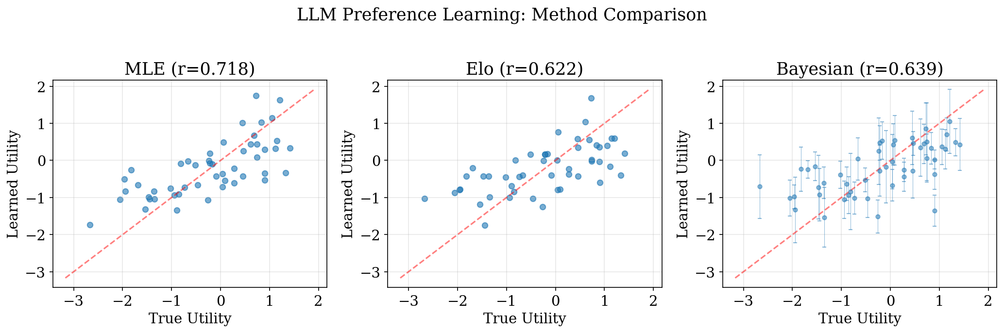
All three methods successfully recover utilities correlated with ground truth
Bayesian provides credible intervals (error bars); MLE and Elo give point estimates

Practical Considerations

Data scale: Production has 10K–100K+ comparisons; MCMC becomes expensive
Cold start: New responses have no history; need initialization strategies
Computational cost: MLE or online methods preferred at scale
Temporal drift: User preferences evolve; online methods naturally adapt
Label noise: All methods are robust to moderate noise ($$10%)

Connection to DPO

DPO for language models is Bradley-Terry MLE where the “utility” is:

\[ r(x, y) = \beta \log \frac{\pi_\theta(y \mid x)}{\pi_{\text{ref}}(y \mid x)} \]

All techniques from this chapter directly apply:

Regularization prevents overfitting to preference data
Adam + LR schedules accelerate training
Cross-validation tunes hyperparameters ($\beta$, learning rate)

Rafailov et al. (2023)

Summary (1)

MLE: Find parameters maximizing data likelihood; gradient = sum of residuals
Bayesian (MCMC): Place prior, sample posterior via Metropolis-Hastings; provides uncertainty
GP + Laplace: Nonparametric reward functions; Gaussian approximation at posterior mode
Fisher information: $W_{ii} = p_i(1-p_i)$ — uncertain comparisons are most informative

Summary (2)

Online (Elo): SGD on BT log-likelihood; K-factor = learning rate; ideal for streaming
Regularization: L2 penalty creates bias-variance tradeoff; equivalent to MAP with Gaussian prior
Cross-validation: K-fold for reliable evaluation and hyperparameter tuning
Adam: Default optimizer; adaptive learning rates; faster than vanilla GD

Key Connections

L2 regularization $=$ MAP with Gaussian prior $\mathcal{N}(0, 1/\lambda)$
Elo $=$ SGD on Bradley-Terry log-likelihood
Fisher information $=$ Laplace approximation precision matrix $W$
DPO $=$ Bradley-Terry MLE on policy log-ratios

These connections unify the chapter: all methods estimate the same model, differing only in computation, data access, and uncertainty quantification.

References

Bradley and Terry (1952)
Elo (1978)
Kingma and Ba (2014)
Rafailov et al. (2023)
Christiano et al. (2017)
Additional:
- Herbrich, Minka, and Graepel (2006)
- Hunter (2004)
- Caron and Doucet (2012)
- Murphy (2012)
- Hastie, Tibshirani, and Friedman (2009)

Bradley, Ralph Allan, and Milton E Terry. 1952. “Rank Analysis of Incomplete Block Designs: I. The Method of Paired Comparisons.” Biometrika 39 (3/4): 324–45.

Caron, François, and Arnaud Doucet. 2012. “Efficient Bayesian Inference for Generalized Bradley-Terry Models.” Journal of Computational and Graphical Statistics 21 (1): 174–96.

Christiano, Paul F, Jan Leike, Tom Brown, Miljan Martic, Shane Legg, and Dario Amodei. 2017. “Deep Reinforcement Learning from Human Preferences.” Advances in Neural Information Processing Systems 30.

Elo, Arpad E. 1978. The Rating of Chessplayers, Past and Present. New York: Arco Publishing.

Hastie, Trevor, Robert Tibshirani, and Jerome Friedman. 2009. The Elements of Statistical Learning: Data Mining, Inference and Prediction. 2nd ed. New York: Springer.

Herbrich, Ralf, Tom Minka, and Thore Graepel. 2006. “TrueSkill: A Bayesian Skill Rating System.” In Advances in Neural Information Processing Systems, 19:569–76.

Hunter, David R. 2004. “MM Algorithms for Generalized Bradley-Terry Models.” The Annals of Statistics 32 (1): 384–406. https://doi.org/10.1214/aos/1079120141.

Kingma, Diederik P., and Jimmy Ba. 2014. “Adam: A Method for Stochastic Optimization.” arXiv Preprint arXiv:1412.6980.

Murphy, Kevin P. 2012. Machine Learning: A Probabilistic Perspective. Cambridge, MA: MIT Press.

Rafailov, Rafael, Archit Sharma, Eric Mitchell, Stefano Ermon, Christopher D. Manning, and Chelsea Finn. 2023. “Direct Preference Optimization: Your Language Model Is Secretly a Reward Model.” https://arxiv.org/abs/2305.18290.