Machine Learning from Human Preferences
Chapter 1: Foundations
Overview
- This chapter lays the theoretical foundation for modeling and predicting choice behavior
- Historical roots: Thurstone (1920s), Luce (1959), Bradley & Terry (1952), McFadden (Nobel 2000)
- Central question: Why is the Bradley-Terry model a reasonable assumption? Where does it come from? When does it fail?
![]()
Preference Learning Across ML
Preference data appears throughout machine learning:
- Recommender systems: clicks, purchases, ratings reveal \(A \succ B\)
- Information retrieval: search click on result 3 \(\Rightarrow\) preferred over results 1, 2
- Robotics & control: preferences over trajectories (smooth > jerky)
- Language model alignment: annotators compare candidate outputs
- Game playing: Elo ratings = Bradley-Terry model for match outcomes
Despite the diversity, all share a common mathematical structure: pairwise comparisons or choices from sets that reveal underlying preferences.
Application: Marketing & Recommender Systems
- Predict demand for new products before production
- What features affect a car purchase?
![]()
Application: Economics & Transportation
- Microeconomics: Random Utility Theory; McFadden: 2000 Nobel Prize
- Transportation: Predicted BART demand before it was built
Application: RL, Robotics, and Language Models
- Robotics: Preferences over trajectories guide policy learning
- LLM alignment: Human feedback drives RLHF and DPO
- Game playing: Elo \(\equiv\) Bradley-Terry for match outcomes
![]()
https://openai.com/research/learning-to-summarize-with-human-feedback
Running Example: LLM Alignment
Modern LLMs are trained in two phases:
- Pretraining: Next-token prediction (cross-entropy loss)
- Proper scoring rule \(\Rightarrow\) calibrated probabilities
- Produces capable models, but not aligned ones
- Posttraining (Alignment): Learn which outputs humans prefer
- RLHF: Collect preferences \(\rightarrow\) train reward model \(\rightarrow\) optimize policy
- DPO: Skip explicit reward model, optimize directly on preferences
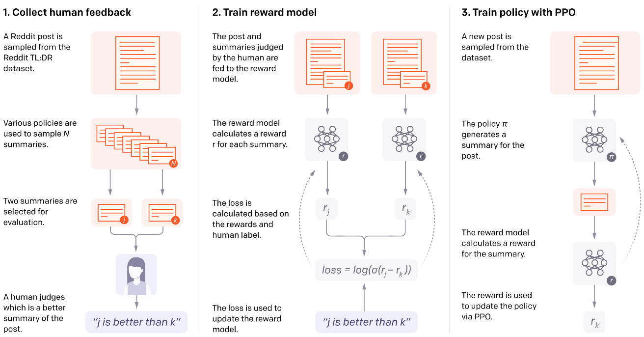
RLHF Pipeline
![]()
Choice models in RL
Three steps:
- Collect preference data: Sample pairs of responses, ask which is better
- Train a reward model: \(r_\phi(x, y)\) predicts human preference
- Optimize the policy: Fine-tune LM to maximize reward (with KL constraint)
Random Preferences
- Items \(j \in \{1, \ldots, M\}\) (products, trajectories, LM responses)
- Preferences: random draws of total orders \(\prec\) (total + transitive)
- Full distribution: \((M!-1)\)-dimensional vector
Goal: Reduce this complexity \(\Rightarrow\) IIA collapses it to \(M\) parameters
Why Stochastic Preferences?
- Deterministic preferences are clean but fail with noisy data
- Even with randomness, assumptions like transitivity and IIA are strong yet practical
Three interpretations of randomness:
- Heterogeneity: Different decision-makers have different utilities (Economics/IO view)
- Bounded rationality: Errors in optimizing utilities (Behavioral view)
- Designer belief: Uncertainty about true preferences (Bayesian view)
Types of Comparison Data (1)
Full preference lists: \(L = (j_1, j_2, \ldots, j_M)\) where \(j_1 \succ j_2 \succ \cdots \succ j_M\)
- Most informative, but cognitive load is high
Choices from subsets: \((j, \mathcal{S})\) — \(j\) is the best from subset \(\mathcal{S}\)
\[
p(j \mid \mathcal{S}) = \sum_{\prec: j \succ k \; \forall k \in \mathcal{S} \setminus \{j\}} p(\prec)
\]
Binary comparisons: \(\mathcal{S} = \{j, j'\}\), write \(Y_{jj'} = 1\)
- Convenient, quick to elicit
- Prominently used in LLM finetuning and evaluation
Types of Comparison Data (2)
Item-wise responses: \(Y_{ij} \in \{0,1\}\) — user \(i\)’s response to item \(j\)
- \(Y_{ij} = 1\): acceptance (like, purchase, engagement)
- \(Y_{ij} = 0\): rejection
Examples: e-commerce purchases, streaming play/skip, dating swipes, content moderation
Outside option: Accept/reject framing with item \(0\)
- \(Y_{j0} = 1\): accepting item \(j\)
- \(Y_{j0} = 0\): rejecting item \(j\)
The Response Matrix
\(N\) users \(\times\) \(M\) items yields an \(N \times M\) response matrix \(Y\) with entries \(Y_{ij} \in \{0, 1\}\):
\[
Y = \begin{bmatrix} Y_{11} & \cdots & Y_{1M} \\ \vdots & \ddots & \vdots \\ Y_{N1} & \cdots & Y_{NM} \end{bmatrix}
\]
- Item-wise: every user-item interaction is one data point — \(O(M)\) per user
- Pairwise: \(O(M^2)\) possible comparisons — more expensive to collect
Comparison Data Across Domains
| Recommender systems |
Choice from set |
Sees \(\{A,B,C\}\), clicks \(B\) |
| Information retrieval |
Implicit pairwise |
Click result 3 \(\Rightarrow\) pref. over 1, 2 |
| LLM alignment |
Binary comparison |
Annotator: \(A \succ B\) |
| Sports/Chess |
Pairwise |
Player \(j\) beats \(k\) |
| Streaming |
Item-wise |
Play (1) or skip (0) |
Goal: learn the underlying utility function from observed choices.
Deterministic Utility Models
When different users have different preferences, we need both user and item parameters:
\[
p(Y_{ij} = 1) = \sigma(H_{ij}), \quad H_{ij} = f(U_i, V_j)
\]
- \(U_i\): user \(i\)’s characteristics
- \(V_j\): item \(j\)’s characteristics
- Stochasticity enters through Bernoulli sampling \(Y_{ij} \sim \text{Bernoulli}(\sigma(H_{ij}))\)
- The function \(f\) and dimensionality of \(U_i, V_j\) define different model families
The Rasch Model
The simplest factor model — \(f\) is additive:
\[
p(Y_{ij} = 1 \mid U_i, V_j) = \sigma(U_i + V_j)
\]
- \(U_i \in \mathbb{R}\): user appetite — general tendency to accept items
- High \(U_i\): enthusiastic user; Low \(U_i\): selective user
- \(V_j \in \mathbb{R}\): item appeal — how universally appealing item \(j\) is
- High \(V_j\): crowd-pleaser; Low \(V_j\): niche item
- Acceptance depends only on the sum \(U_i + V_j\)
Rasch Implies Bradley-Terry
For a single user, the Rasch model implies Bradley-Terry for pairwise comparisons:
\[
p(j \succ k \mid i) = \sigma((U_i + V_j) - (U_i + V_k)) = \sigma(V_j - V_k)
\]
The user-specific parameter \(U_i\) cancels out!
| Pairwise \((j \succ k)\) |
Item differences only |
\(V_j - V_k\) (up to constant) |
| Item-wise \((Y_{ij})\) |
User appetites + item appeals |
\(U_i\) and \(V_j\) (up to constant) |
This explains why recommender systems use item-wise data (clicks, purchases) while ranking systems (chess, LLM eval) can use pairwise comparisons.
K-Dimensional Factor Models: Dot-Product
Rasch assumes 1D — users might love action but dislike romance.
Logistic factor model: \(H_{ij} = U_i^\top V_j + Z_j\)
- \(U_i \in \mathbb{R}^K\): user embedding; \(V_j \in \mathbb{R}^K\): item embedding
- \(Z_j \in \mathbb{R}\): item offset (baseline popularity)
- Dot product measures user-item alignment; \(K = 1\) reduces to Rasch
Foundation of Netflix Prize, collaborative filtering, two-tower models.
K-Dimensional Factor Models: Ideal Point
Ideal point model: users prefer items close to their ideal point:
\[
H_{ij} = -\|U_i - V_j\|_2 + Z_j
\]
- Users and items live in the same \(K\)-dimensional space
- Pros: Can learn preferences faster by exploiting geometry
- Cons: Embedding assumption may be strong; must select distance function
Natural for: political preferences (voters vs. candidates), music taste, product specs
Jamieson and Nowak (2011); Tatli, Nowak, and Vinayak (2022)
Two Views of Stochastic Choice
Deterministic utility (Latent variable):
- \(H_{ij} = f(U_i, V_j)\) — fixed
- Randomness in \(Y_{ij} \sim \text{Bernoulli}(\sigma(H_{ij}))\)
- “User has fixed preferences; responses are noisy”
Stochastic utility (Random utility):
- \(\tilde{H}_{ij} = f(U_i, V_j) + \varepsilon_{ij}\)
- Choice: \(j \succ k \iff \tilde{H}_{ij} \gt \tilde{H}_{ik}\)
- “User’s utility evaluation fluctuates”
Both yield \(p(j \succ k \mid i) = \sigma(V_j - V_k)\) for additive \(f\) — observationally equivalent for pairwise data.
Stochastic Utility Models
Random utility: \(\tilde{H}_j = V_j + \varepsilon_j\)
- \(V_j\): mean utility (deterministic)
- \(\varepsilon_j\): noise (stochastic), typically independent across items
Three interpretations of noise:
- Heterogeneity of decision-makers (Economics/IO)
- Errors in optimization of utilities (Bounded Rationality)
- Designer’s belief about preferences (Bayesian)
The key simplifying assumption: when \(\varepsilon_j\) are i.i.d. \(\Rightarrow\) IIA
Binary Choice Models
Binary choice with individual attributes
\[
\begin{cases}
U_n = \beta s_n + \epsilon_n \\
y_n =
\begin{cases}
1 & U_n \gt 0 \\
0 & U_n \leq 0
\end{cases}
\end{cases}
\]
- \(\epsilon \sim\) Logistic: \(P_{n1} = \frac{1}{1 + \exp(-\beta s_n)}\)
- \(\epsilon \sim\) Standard Normal (probit): \(P_{n1} = \Phi(\beta s_n)\)
Bradley-Terry Model
Utility depends on alternative attributes with extreme value noise:
\[
\begin{cases}
U_{n1} = \beta z_{n1} + \epsilon_{n1} \\
U_{n2} = \beta z_{n2} + \epsilon_{n2} \\
\epsilon_{n1}, \epsilon_{n2} \sim \text{iid extreme value}
\end{cases}
\] \[
\Rightarrow \quad P_{n1} = \frac{\exp(\beta z_{n1})}{\exp(\beta z_{n1}) + \exp(\beta z_{n2})} = \frac{1}{1 + \exp(-\beta (z_{n1} - z_{n2}))}
\]
- Gaussian noise alternative: \(P_{n1} = \Phi(\beta (z_{n1} - z_{n2}))\)
Multiple Alternatives (Softmax)
With \(J\) alternatives and extreme value noise:
\[
\begin{cases}
U_{ni} = \beta z_{ni} + \epsilon_{ni} \\
\epsilon_{ni} \sim \text{iid extreme value}
\end{cases} \quad \Rightarrow \quad P_{ni} = \frac{\exp(\beta z_{ni})}{\sum_{j=1}^{J} \exp(\beta z_{nj})}
\]
- Equivalent to multiclass logistic regression (multinomial logit)
- Can also replace noise model with Gaussians (multinomial probit)
Plackett-Luce (Rankings)
The Plackett-Luce model extends to full rankings as a sequence of choices:
\[
Pr(\text{ranking } 1, 2, \dots, J) = \prod_{m=1}^{J-1} \frac{\exp(\beta z_m)}{\sum_{j=m}^{J} \exp(\beta z_{nj})}
\]
- Also known as: rank ordered logit, exploded logit
- All extensions apply: nonlinear utility, correlated noise, etc.
Estimation
- Linear case: Maximum likelihood estimators (logistic and probit regression)
- Complex function classes: Regularized ML with SGD
- Standard tradeoffs: Bias-variance tradeoff
- More complex models generally require more data
- Most ML applications pool data across individuals whose differences may matter
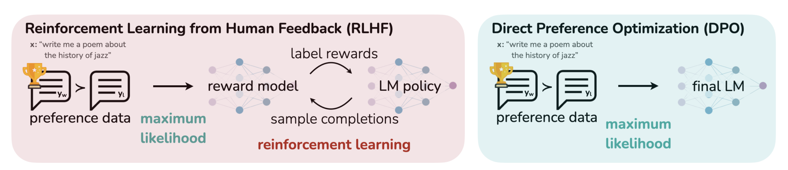
Why DPO?
![]()
DPO vs PPO
- RLHF pipeline is complex and unstable due to the reward model optimization.
- DPO is more stable and can be used to optimize the reward model directly.
Rafailov et al. (2023)
DPO: Bradley-Terry model
- Given prompt \(x\) and completions \(y_w\) and \(y_l\) the choice model gives the preference
\[
p^*(y_w \succ y_l \mid x) = \frac{\exp(r^*(x, y_w))}{\exp(r^*(x, y_w)) + \exp(r^*(x, y_l))}
\]
where \(r^*(x, y)\) is some latent reward model that we do not have access to (i.e., the human preference)
DPO: Bradley-Terry model
Luckily, we can use parameterize the reward model with some neural networks with parameters \(\phi\):
Let us start with the Reward Maximization Objective in RL: \[
\max_{\pi_\theta} \mathbb{E}_{x \sim \mathcal{D}, y \sim \pi_\theta(y|x)} [r_\phi(x, y) - \beta D_{KL}(\pi_\theta(y|x) \| \pi_{\text{ref}}(y|x))]
\]
- Where \(\pi_\theta(y|x)\) is the language model, and \(\pi_{\text{ref}}(y|x)\) is the reference model (e.g., the language model before fine-tuning)
\[
\max_{\pi_\theta} \mathbb{E}_{x \sim \mathcal{D}, y \sim \pi_\theta(y|x)} [r_\phi(x, y) - \beta D_{KL}(\pi_\theta(y|x) \| \pi_{\text{ref}}(y|x))]
\]
Recall the definition of KL divergence: \[
D_{KL}(p \| q) = \sum_{x \in \mathcal{X}} p(x) \log \frac{p(x)}{q(x)} = \mathbb{E}_{x \sim \mathcal{X}} \left[ \log \frac{p(x)}{q(x)} \right]
\]
Substituting the KL divergence, we can rewrite the objective as: \[
\begin{aligned}
&\max_{\pi_\theta} \mathbb{E}_{x \sim \mathcal{D}, y \sim \pi_\theta(y|x)} \left[ r_\phi(x, y) - \beta \mathbb{E}_{y \sim \pi_\theta(y|x)} \left[\log \frac{\pi_\theta(y|x)}{\pi_{\text{ref}}(y|x)} \right] \right]\\
&=\max_{\pi_\theta} \mathbb{E}_{x \sim \mathcal{D}} \mathbb{E}_{y \sim \pi_\theta(y|x)} \left[ r_\phi(x, y) - \beta \log \frac{\pi_\theta(y|x)}{\pi_{\text{ref}}(y|x)} \right]
\end{aligned}
\]
Then, we can continue to derive the objective as: \[
\begin{aligned}
&\max_{\pi_\theta} \mathbb{E}_{x \sim \mathcal{D}} \mathbb{E}_{y \sim \pi_\theta(y|x)} \left[ r_\phi(x, y) - \beta \log \frac{\pi_\theta(y|x)}{\pi_{\text{ref}}(y|x)} \right] \\
&\propto \min_{\pi_\theta} \mathbb{E}_{x \sim \mathcal{D}} \mathbb{E}_{y \sim \pi_\theta(y|x)} \left[ \log \frac{\pi_\theta(y|x)}{\pi_{\text{ref}}(y|x)} - \frac{1}{\beta} r_\phi(x, y) \right]\\
&= \min_{\pi_\theta} \mathbb{E}_{x \sim \mathcal{D}} \mathbb{E}_{y \sim \pi_\theta(y|x)} \left[ \log \frac{\pi_\theta(y|x)}{\frac{1}{Z(x)} \pi_{\text{ref}}(y|x) \exp\left(\frac{1}{\beta} r_\phi(x, y)\right)} - \log Z(x) \right]
\end{aligned}
\] where \(Z(x) = \sum_{y} \pi_{\text{ref}}(y|x) \exp\left(\frac{1}{\beta} r_\phi(x, y)\right)\)
Because \(Z(x)\) is a constant with respect to \(\pi_\theta\), we can define: \[
\pi^*(y|x) = \frac{1}{Z(x)} \pi_{\text{ref}}(y|x) \exp\left(\frac{1}{\beta} r_\phi(x, y)\right)
\]
Then, we can rewrite the optimization problem as: \[
\begin{aligned}
&\min_{\pi_\theta} \mathbb{E}_{x \sim \mathcal{D}} \mathbb{E}_{y \sim \pi_\theta(y|x)} \left[ \log \frac{\pi_\theta(y|x)}{\pi^*(y|x)} - \log Z(x) \right]\\
&\quad = \mathbb{D}_{KL}\!\left(\pi_\theta(y|x) \,\|\, \pi^*(y|x)\right) - \log Z(x)
\end{aligned}
\]
Thus, the optimal solution (i.e., the optimal language model) is: \[
\pi_\theta(y|x) = \pi^*(y|x) = \frac{1}{Z(x)} \pi_{\text{ref}}(y|x) \exp\left(\frac{1}{\beta} r_\phi(x, y)\right)
\]
With some algebra, we can show that the optimal reward model is: \[
\begin{aligned}
\pi_\theta(y|x) &= \frac{1}{Z(x)} \pi_{\text{ref}}(y|x) \exp\left(\frac{1}{\beta} r_\phi(x, y)\right)\\
\log \pi_\theta(y|x) &= \log \pi_{\text{ref}}(y|x) + \frac{1}{\beta} r_\phi(x, y) - \log Z(x) \text{// perform } \log(.)\\
r_\phi(x, y) &= \beta \log \frac{\pi_\theta(y|x)}{\pi_{\text{ref}}(y|x)} + \beta \log Z(x)\\
\end{aligned}
\]
Recall the Bradley-Terry model: \[
p_\phi(y_w \succ y_l \mid x) = \frac{\exp(r_\phi(x, y_w))}{\exp(r_\phi(x, y_w)) + \exp(r_\phi(x, y_l))}
\]
And the optimal reward model: \[
r_\phi(x, y) = \beta \log \frac{\pi_\theta(y|x)}{\pi_{\text{ref}}(y|x)} + \beta \log Z(x)
\]
Substituting, we can rewrite the choice model as: \[
\begin{aligned}
p_\phi(y_w \succ y_l \mid x) &= \frac{1}{1 + \exp\left( \beta \log \frac{\pi_\theta(y_l | x)}{\pi_{\text{ref}}(y_l | x)} - \beta \log \frac{\pi_\theta(y_w | x)}{\pi_{\text{ref}}(y_w | x)} \right)}\\
&= \sigma\left( \beta \log \frac{\pi_\theta(y_w | x)}{\pi_{\text{ref}}(y_w | x)} - \beta \log \frac{\pi_\theta(y_l | x)}{\pi_{\text{ref}}(y_l | x)} \right)
\end{aligned}
\]
DPO: Bradley-Terry model
The reward model loss maximizes the likelihood of the choice model: \[
\mathcal{L} (r_\theta, \mathcal{D}) = - \mathbb{E}_{(x, y_w, u_l) \sim \mathcal{D}} \left[ \log p_\phi(y_w \succ y_l \mid x) \right]
\]
DPO Loss
Substituting the optimal reward, we obtain the DPO loss:
\[
\mathcal{L}_{DPO}(\pi_\theta; \pi_{\text{ref}}) = -\mathbb{E}_{(x, y_w, y_l) \sim D} \left[ \log \sigma\left( \beta \log \frac{\pi_\theta(y_w | x)}{\pi_{\text{ref}}(y_w | x)} - \beta \log \frac{\pi_\theta(y_l | x)}{\pi_{\text{ref}}(y_l | x)} \right) \right]
\]
Rafailov et al. (2023)
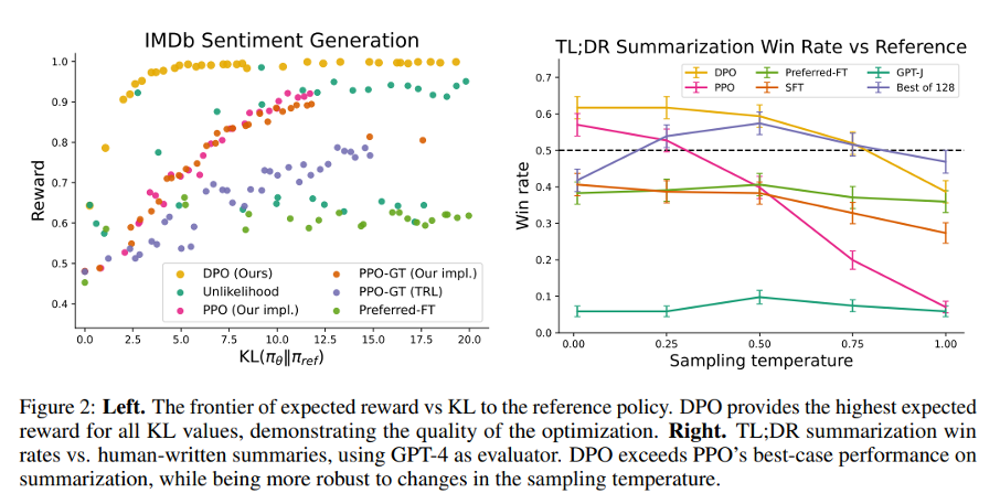
![]()
RLHF Comparison
Independence of Irrelevant Alternatives (IIA)
IIA assumes the relative likelihood of choosing \(j\) vs \(k\) is unchanged by a third alternative \(\ell\):
\[
\frac{p(j \mid \mathcal{S})}{p(k \mid \mathcal{S})} = \frac{p(j \mid \mathcal{S} \cup \{\ell\})}{p(k \mid \mathcal{S} \cup \{\ell\})}
\]
- Introduced by Luce (1959)
- Reduces \((M!-1)\) parameters to just \(M\) parameters
- Makes learning feasible!
IIA-Gumbel Equivalence
Theorem 1: A random utility model \(H_j\) satisfies IIA if and only if \(H_j = V_j + \varepsilon_j\) where \(\varepsilon_j\) are i.i.d. Gumbel distributed.
- Gumbel CDF: \(F(x) = e^{-e^{-x}}\)
IIA-Gumbel Equivalence: Proof Sketch
(⇐) Gumbel \(\Rightarrow\) IIA: \[
\frac{p(j \mid \mathcal{S})}{p(k \mid \mathcal{S})} = \frac{e^{V_j}/\sum_{\ell} e^{V_\ell}}{e^{V_k}/\sum_{\ell} e^{V_\ell}} = e^{V_j - V_k}
\] Independent of \(\mathcal{S}\) — IIA holds.
(⇒) IIA \(\Rightarrow\) Gumbel: IIA forces multiplicative structure; only Gumbel is compatible (Yellott, 1977).
Choice Probabilities under IIA
Theorem 2: Under IIA (\(H_j = V_j + \varepsilon_j\), i.i.d. Gumbel), the probabilities are:
Choices from sets (softmax): \[
p(j \mid \mathcal{S}) = \frac{e^{V_j}}{\sum_{k \in \mathcal{S}} e^{V_k}} = \operatorname{softmax}_j ((V_k)_{k \in \mathcal{S}})
\]
Binary comparisons (Bradley-Terry): \[
p(Y_{jj'} = 1) = \sigma(V_j - V_{j'}) = \frac{1}{1 + e^{-(V_j - V_{j'})}}
\]
Choice Probabilities under IIA (cont.)
Full rankings (Plackett-Luce): \[
p(j_1 \succ \cdots \succ j_M) = \prod_{m=1}^{M-1} \frac{e^{V_{j_m}}}{\sum_{k=m}^{M} e^{V_{j_k}}}
\]
Example: \(V = (0, 1, 2)\)
- \(p(3 \succ 1) = \sigma(2) \approx 0.88\)
- \(p(\cdot \mid \{1,2,3\}) \approx (0.09, 0.24, 0.67)\)
Many Names, One Model
All are special cases of random utility with i.i.d. Gumbel noise under IIA:
| Binary comparisons |
Bradley-Terry |
| Full rankings |
Plackett-Luce |
| Accept/reject |
Logistic regression |
| Choices from subsets |
Logit model |
| Multi-class |
Multinomial logit |
IIA Justifies DPO
DPO assumes Bradley-Terry: \(p(y \succ y' \mid x) = \sigma(r(x,y) - r(x,y'))\)
Justified by IIA: humans compare implicit rewards with i.i.d. Gumbel noise.
When BT fails for DPO:
- Context effects: preferences depend on what other options are shown
- Intransitive preferences: \(A \succ B \succ C \succ A\)
- Annotator disagreement: mixture model needed
Identification Problem
Different utility vectors can generate identical choice probabilities:
\[
\frac{e^{V_j + c}}{\sum_{k \in \mathcal{S}} e^{V_k + c}} = \frac{e^c \cdot e^{V_j}}{e^c \cdot \sum_{k} e^{V_k}} = \frac{e^{V_j}}{\sum_{k} e^{V_k}}
\]
Implications:
- Normalization required: Must fix one value (e.g., \(V_0 = 0\))
- Only differences matter: Can only identify \(V_j - V_k\), not absolute levels
- Connection to DPO: The reference policy \(\pi_{\text{ref}}\) provides normalization
- Implicit reward: \(r^*(x,y) = \beta \log \frac{\pi_\theta(y|x)}{\pi_{\text{ref}}(y|x)}\)
The Rashomon Effect
Even after identification, many structurally different models can fit data equally well. Named after Kurosawa’s 1950 film.
Example: 100 pairwise comparisons, 5 items — all achieve 90% accuracy:
- Bradley-Terry with utilities \((0, V_2, V_3, V_4, V_5)\)
- 2-group mixture with group-specific utilities
- Nested logit with correlation parameters
For alignment: Many reward functions explain human feedback equally well — which one should we optimize?
Connecting Item-wise and Pairwise Models
Rasch \(\rightarrow\) Bradley-Terry: User params cancel (\(U_i\) disappears)
General factor model: \(p(j \succ k \mid i) = \sigma\left(U_i^\top (V_j - V_k) + (Z_j - Z_k)\right)\)
- This is not standard BT — preference depends on user \(U_i\)!
- Different users may rank the same items differently
When Do User Params Cancel?
User-specific parameters \(U_i\) cancel when:
- Rasch model (additive structure)
- Single user (\(N = 1\))
- Homogeneous population (\(U_i = U\) for all \(i\))
Use BT for ranking items globally; factor models for personalization.
IIA Limitation: Population Heterogeneity
Sub-populations satisfying IIA \(\not\Rightarrow\) full population satisfies IIA
Mixture model: \[
p(Y_{jj'} = 1) = \sum_{i=1}^N \alpha_i \, \sigma(V_j^{(i)} - V_{j'}^{(i)})
\]
Intuition: A mixture of Gumbels is not Gumbel (like a mixture of Gaussians is not Gaussian)
Solution: Random coefficients logit \(V_j = \beta^\top x_j + \varepsilon_j\), \(\beta \sim N(\mu, \Sigma)\)
IIA Limitation: Red Bus / Blue Bus
Items 1, 2 are nearly identical (red bus, blue bus); item 3 is different (train).
Under IIA with \(V_1 = V_2\):
- Adding the clone reduces \(p(\text{train} \mid \{1,2,3\})\) vs \(p(\text{train} \mid \{1,3\})\)
- Intuitively, demand for train should be unchanged!
The fix: Allow correlated noise between similar alternatives
\[
\begin{aligned}
&\bigl(p(1 \mid \{1,2,3\}),\; p(2 \mid \{1,2,3\}),\; p(3 \mid \{1,2,3\})\bigr)\\
&\quad = \left(\tfrac{p(1 \mid \{1,3\})}{2},\; \tfrac{p(2 \mid \{2,3\})}{2},\; p(3 \mid \{1,3\})\right)
\end{aligned}
\]
when errors for items 1, 2 are perfectly correlated.
Beyond Bradley-Terry (1)
- Probit: Gaussian noise \(\varepsilon \sim \mathcal{N}(0, \Sigma)\)
- Allows arbitrary correlations; handles red-bus/blue-bus
- Disadvantage: no closed-form choice probabilities
- Nested logit: Group alternatives into “nests” with within-nest correlation
- IIA within nests, substitution across nests
Beyond Bradley-Terry (2)
- Mixed logit (random coefficients): \(\beta \sim F\)
- Can approximate any random utility model (McFadden and Train 2000)
- Gaussian Processes: Nonparametric, nonlinear reward \(r(x) \sim \mathcal{GP}(m, k)\)
- RBF kernel: \(k(x,x') = \sigma_f^2 \exp(-\|x-x'\|^2 / 2\ell^2)\)
- Useful when linear rewards are too restrictive
Summary (1)
- Preference data is ubiquitous in ML: recommenders, IR, robotics, LLMs
- Random preferences: \((M!-1)\) parameters — intractable without simplification
- IIA reduces complexity to \(M\) parameters \(\Rightarrow\) i.i.d. Gumbel noise
- Bradley-Terry: \(p(j \succ k) = \sigma(V_j - V_k)\) — arises from IIA
Summary (2)
- Rasch model connects item-wise and pairwise data; user params cancel
- DPO assumes BT, justified by IIA; full derivation from RL objective
- Limitations: heterogeneity (mixtures), red-bus/blue-bus (cloning), identification, Rashomon effect
- Extensions: probit, nested logit, mixed logit, GPs