Machine Learning from Human Preferences
Chapter 4: Preferential Bayesian Optimization
1. Preliminary
Which looks more like fire? Left or Right?
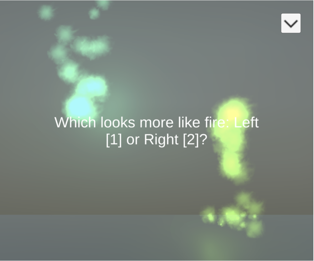
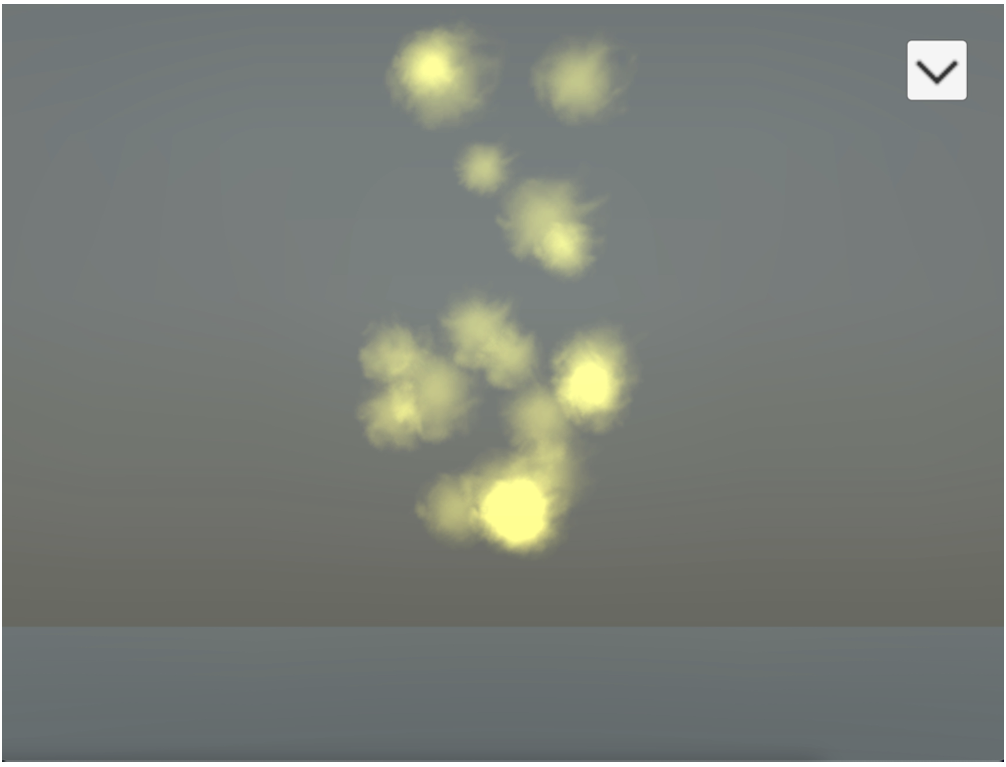
Astudillo et al. (2023)
1. Preliminary
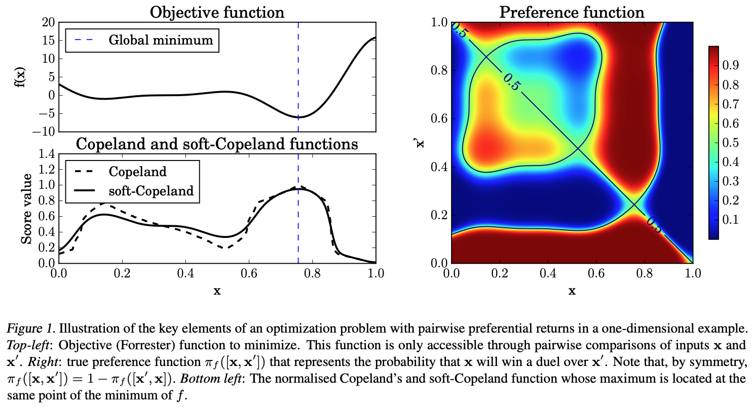
Let \(\mathcal{X} \subseteq \mathbb{R}^q\) be a set of points and \(g: \mathcal{X} \rightarrow \mathbb{R}\) be a black-box function. Our objective is to find
\[
x_{\text{min}} = \arg \min_{x \in \mathcal{X}} g(x)
\]
where \(g\) is not directly accessible, and queries can only be performed in pairs of points, referred to as duels \([x, x'] \in \mathcal{X} \times \mathcal{X}\).
The feedback is binary \(y \in \\{0, 1\\}\). \(y = 1\) if \(x\) is preferred (lower value) and \(y = 0\) otherwise. The goal is to find \(x_{\text{min}}\) with the minimal number of query.
González et al. (2017)
1. Preliminary
Recall \[
p(x \succ x') = \sigma(r(x') - r(x))
\] where \(r(\cdot)\) and \(\sigma(\cdot)\) is the latent reward function and sigmoid function, respectively. We want to find \(x\) that can minimize \(g(\cdot)\), so that \(r(x) = -g(x)\). Hence, \(p(x \succ x') = \sigma(g(x) - g(x'))\).
For any duel \([x, x']\), we have \[p(x \succ x') \geq 0.5 \iff g(x) \leq g(x')\]
González et al. (2017)
1. Preliminary: Copeland score
The Copeland score is used to measure how often an option wins in pairwise comparisons against others. The normalized Copeland score is defined as: \[S(x) = \text{Vol}(\mathcal{X})^{-1} \int_{\mathcal{X}} \mathbb{I}(g(x) \leq g(x')) dx'
\] where \(\text{Vol}(\mathcal{X})\) normalizes the score to \([0, 1]\).
Zoghi et al. (2015); Nurmi (1983)
1. Preliminary: Copeland score
The normalized Copeland score is not smooth nor differentiable, motivating the soft version of it: \[
\begin{aligned}
C(x) \propto \int_{\mathcal{X}} \sigma(g(x') - g(x)) dx' = \int_{\mathcal{X}} p(x \succ x') dx'
\end{aligned}
\]
- If \(x_C\) is preferred to all other points (i.e. Condorcet winner), then \(C(x_C) = 1\), which is maximized.
- This implies that by observing the results of a set of duels, we can solve the original optimization problem by finding Condorcet winner of Copeland score.
González et al. (2017)
1. Preliminary
González et al. (2017)
2. Learning Latent Score Function
- For convenience, we rewrite \(p(x \succ x')\) as \(\pi([x, x'])\). We have already observed \(N\) duels in \(\mathcal{D} = \\{([x_1, x_1'], y_1), \\dots, ([x_N, x_N'], y_N)\\}\).
- We want to learn \(\pi([x, x'])\) so that for new coming duels \([x_t, x_t']\), we can predict \(y_t\). The process of learning can be summarized as:
- Compute the posterior distribution \(p(f_t | \mathcal{D}, [x_t, x_t'], \theta)\), where \(f_t = g(x_t') - g(x_t)\), \(\theta\) is learning parameters.
- Compute the preference score \(\pi([x_t, x_t'];\mathcal{D},\theta) = \int \left[ \sigma(f_t) p(f_t | \mathcal{D}, [x_t, x_t'], \theta) \right] df_t\).
González et al. (2017)
2. Learning Latent Score Function
The soft Copeland score can be obtained by integrating the preference score over all possible duels. Thus, it is possible to learn this function from data by integrating \(\pi([x, x'], \mathcal{D})\). We can use Monte Carlo sampling to approximate the integral: \[
\begin{aligned}
C(x; \mathcal{D}, \theta) &\propto \int_{\mathcal{X}} \pi([x, x']; \mathcal{D}, \theta) dx' \approx \frac{1}{M} \sum_{i=1}^{M} \pi([x, x_i]; \mathcal{D}, \theta)
\end{aligned}
\] The Condorcet winner is a maximizer of the soft Copeland score found by any suitable optimizer: \(x_C = \arg \max_{x \in \mathcal{X}} C(x; \mathcal{D}, \theta)\) González et al. (2017)
2. Learning Latent Score Function: Probability 101
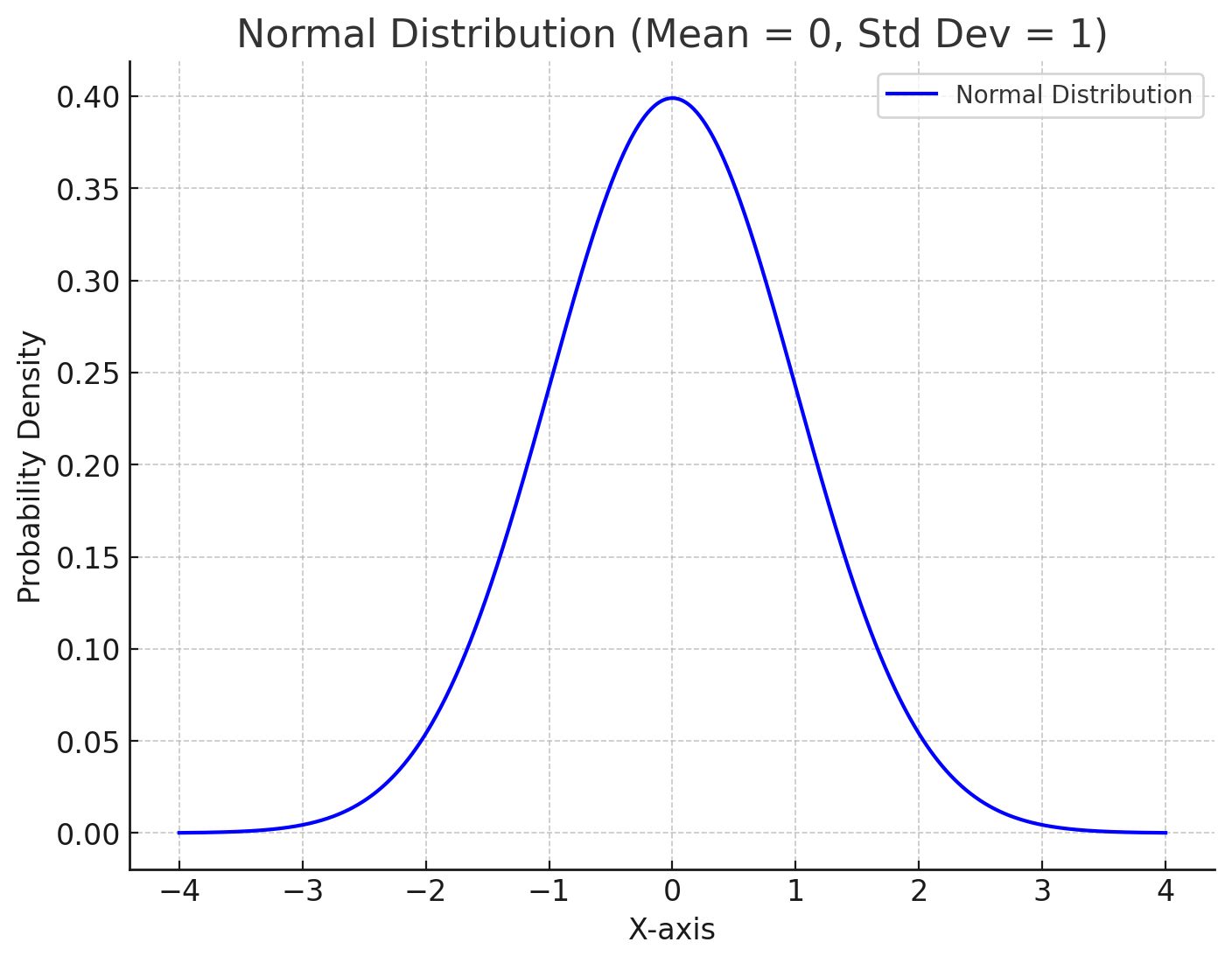
A Gaussian distribution (i.e. normal distribution) is a continuous probability distribution that is completely described with two parameters (mean \(\mu\) and variance \(\sigma^2\)) with the following density: \[
f(x | \mu, \sigma^2) = \frac{1}{\sqrt{2\pi\sigma^2}} \exp\left(-\frac{(x - \mu)^2}{2\sigma^2}\right)
\] 
2. Learning Latent Score Function: Probability 101
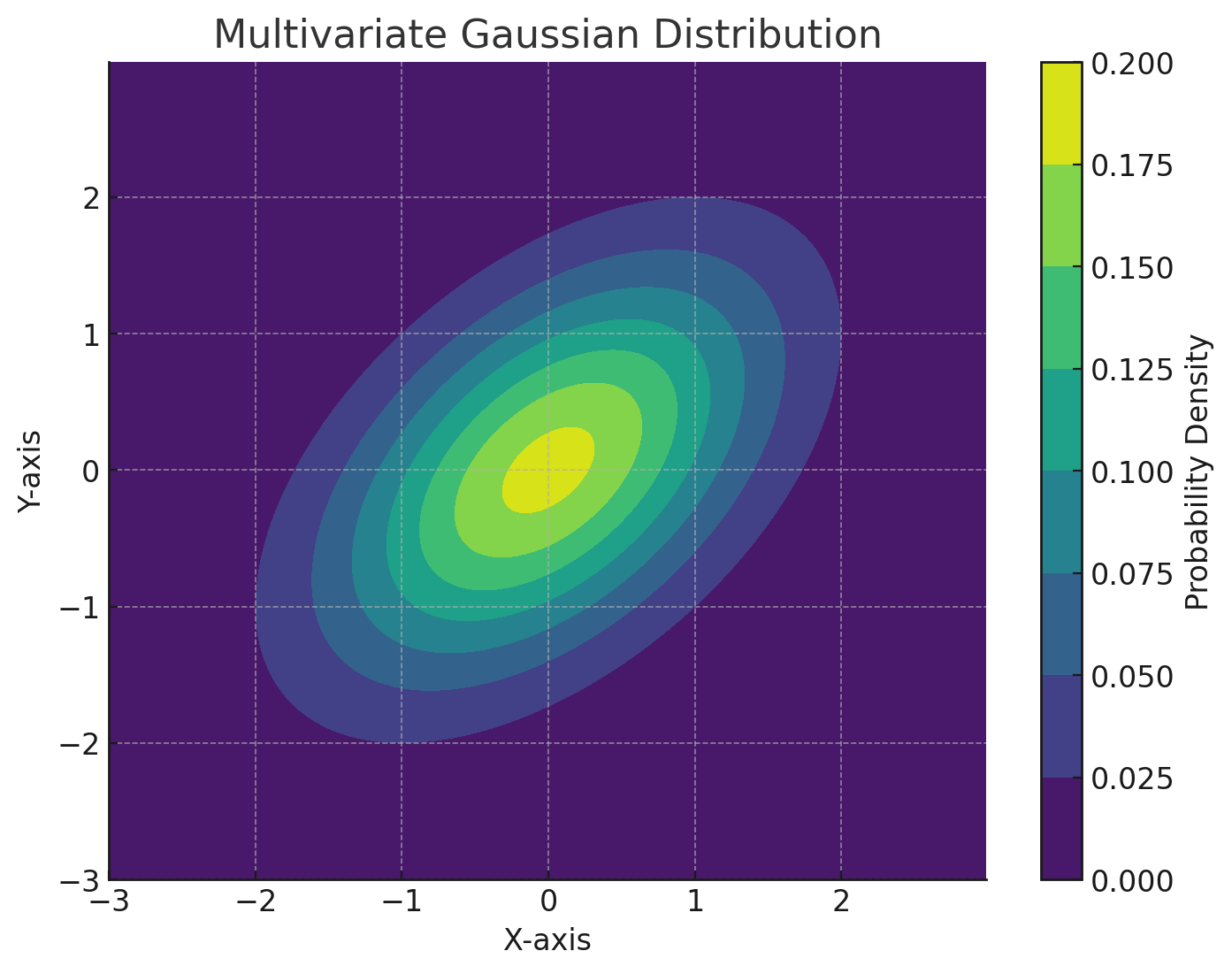
A multivariate Gaussian distribution is a generalization of the one-dimensional Gaussian distribution to higher dimensions by defining a mean vector \(\mu\) and a covariance matrix \(\Sigma\). \[
\Sigma = \begin{bmatrix}
\sigma_{1,1} & \sigma_{1,2} & \cdots & \sigma_{1,d} \\
\sigma_{2,1} & \sigma_{2,2} & \cdots & \sigma_{2,d} \\
\vdots & \vdots & \ddots & \vdots \\
\sigma_{d,1} & \sigma_{d,2} & \cdots & \sigma_{d,d}
\end{bmatrix}
\] where \(\sigma_{i,j} = (x_i - \mu_i)(x_j - \mu_j)\) is the covariance between dimensions \(i\) and \(j\).
2. Learning Latent Score Function: Probability 101
2. Learning Latent Score Function: Probability 101
- Marginalization is a process of obtaining the probability distribution of a subset of random variables from a joint probability distribution.
- For example, given a joint distribution \(P(X, Y)\), the marginal distribution of \(X\) is obtained by summing over all possible values of \(Y\): \[
P(X) = \sum_Y P(X, Y)
\]
2. Learning Latent Score Function: Probability 101
Example: Given a joint distribution \(P(X, Y)\) as follows: \[
\begin{array}{|c|c|c|}
\hline
X & Y & P(X, Y) \\
\hline
0 & 0 & 0.1 \\
0 & 1 & 0.2 \\
1 & 0 & 0.3 \\
1 & 1 & 0.4 \\
\hline
\end{array}
\] Compute the marginal distribution of \(X\)?
2. Learning Latent Score Function: Probability 101
\[
\begin{array}{|c|c|c|}
\hline
X & Y & P(X, Y) \\
\hline
0 & 0 & 0.1 \\
0 & 1 & 0.2 \\
1 & 0 & 0.3 \\
1 & 1 & 0.4 \\
\hline
\end{array}
\] The marginal distribution of \(X\) is obtained by summing over all possible values of \(Y\): \[
P(X) = \sum_Y P(X, Y) = \begin{cases}
0.1 + 0.2 = 0.3 & \text{if } X = 0 \\
0.3 + 0.4 = 0.7 & \text{if } X = 1
\end{cases}
\]
2. Learning Latent Score Function: Probability 101
- Conditioning is a process of obtaining the probability distribution of a random variable given the value of another random variable.
- For example, given a joint distribution \(P(X, Y)\), the conditional distribution of \(X\) given \(Y\) is obtained by dividing the joint distribution by the marginal distribution of \(Y\): \[
P(X | Y) = \frac{P(X, Y)}{P(Y)}
\]
2. Learning Latent Score Function: Probability 101
Example: Given a joint distribution \(P(X, Y)\) as follows: \[
\begin{array}{|c|c|c|}
\hline
X & Y & P(X, Y) \\
\hline
0 & 0 & 0.1 \\
0 & 1 & 0.2 \\
1 & 0 & 0.3 \\
1 & 1 & 0.4 \\
\hline
\end{array}
\] Compute the conditional distribution of \(X\) given \(Y = 1\)?
2. Learning Latent Score Function: Probability 101
The conditional distribution of \(X\) given \(Y = 1\) is obtained by dividing the joint distribution by the marginal distribution of \(Y = 1\): \[
P(X | Y = 1) = \frac{P(X, Y = 1)}{P(Y = 1)} = \begin{cases}
\frac{0.2}{0.2 + 0.4} = 0.33 & \text{if } X = 0 \\
\frac{0.4}{0.2 + 0.4} = 0.67 & \text{if } X = 1
\end{cases}
\]
3. Learning Latent Score Function
When learning a function \(f(x)\) without knowing its functional form, we typically have two modeling choices: - Assume a parametric form for \(f(x)\), e.g., \(f(x) = \theta_0 + \theta_1 x + \theta_2 x^2\) and estimate the parameters \(\theta\) (by using Maximum Likelihood Estimation, for example). - Assume a nonparametric form for \(f(x)\), e.g., \(f(x) \sim \mathcal{GP}(\mu(x), k(x, x'))\), where \(\mu(x)\) is the mean function and \(k(x, x')\) is the kernel function.
3. Learning Latent Score Function: GP
- Gaussian process (GP) is a collection of random variables, any finite number of which have a joint Gaussian distribution. GP learns the underlying distribution of the function \(f(x)\) from training data by modeling the training data \(Y_{\text{train}}\) and test data \(Y_{\text{test}}\) as a multivariate normal distribution.
- The mean function \(\mu\) is often assumed to be 0, simplifying the conditioning process. This can later be adjusted by adding \(\mu\) back during prediction (a process known as centering).
- The covariance matrix \(\Sigma\) defines the relationship between data points, and it is computed using a kernel function \(k(x, x')\). The kernel function is crucial as it determines the smoothness of the function class.
3. Learning Latent Score Function: GP
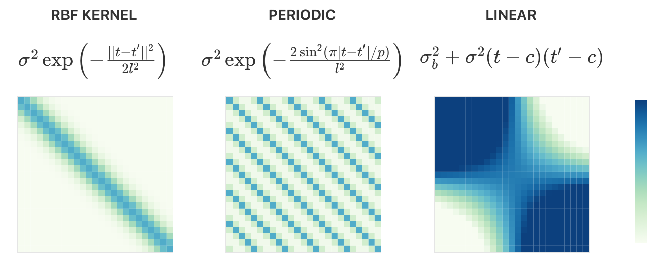
The covariance matrix \(\Sigma\) is computed by applying the kernel function \(k(t,t')\) to each pair of data points: \[
k: \mathbb{R}^n \times \mathbb{R}^n \rightarrow \mathbb{R},\quad
\Sigma = \text{Cov}(X,X') = k(t,t')
\] - Stationary Kernels: Depend only on the relative position of data points. Examples: RBF (Invariant to translation, covariance decays with distance), Periodic (Adds periodicity, controlled by a parameter \(P\)) - Non-stationary Kernels: Depend on the absolute position. Example: Linear (Sensitive to the location of points) - Combining Kernels
3. Learning Latent Score Function: GP
https://distill.pub/2019/visual-exploration-gaussian-processes/
3. Learning Latent Score Function: GP
- Prior Distribution describes the probability of possible functions before observing any training data.
- The covariance matrix of the prior is set up using the kernel function, which determines the types of functions that are more probable within the prior.
- We provide samples from different kernels to highlight how functions are distributed normally around the mean.
3. Learning Latent Score Function: GP
RBF Kernel
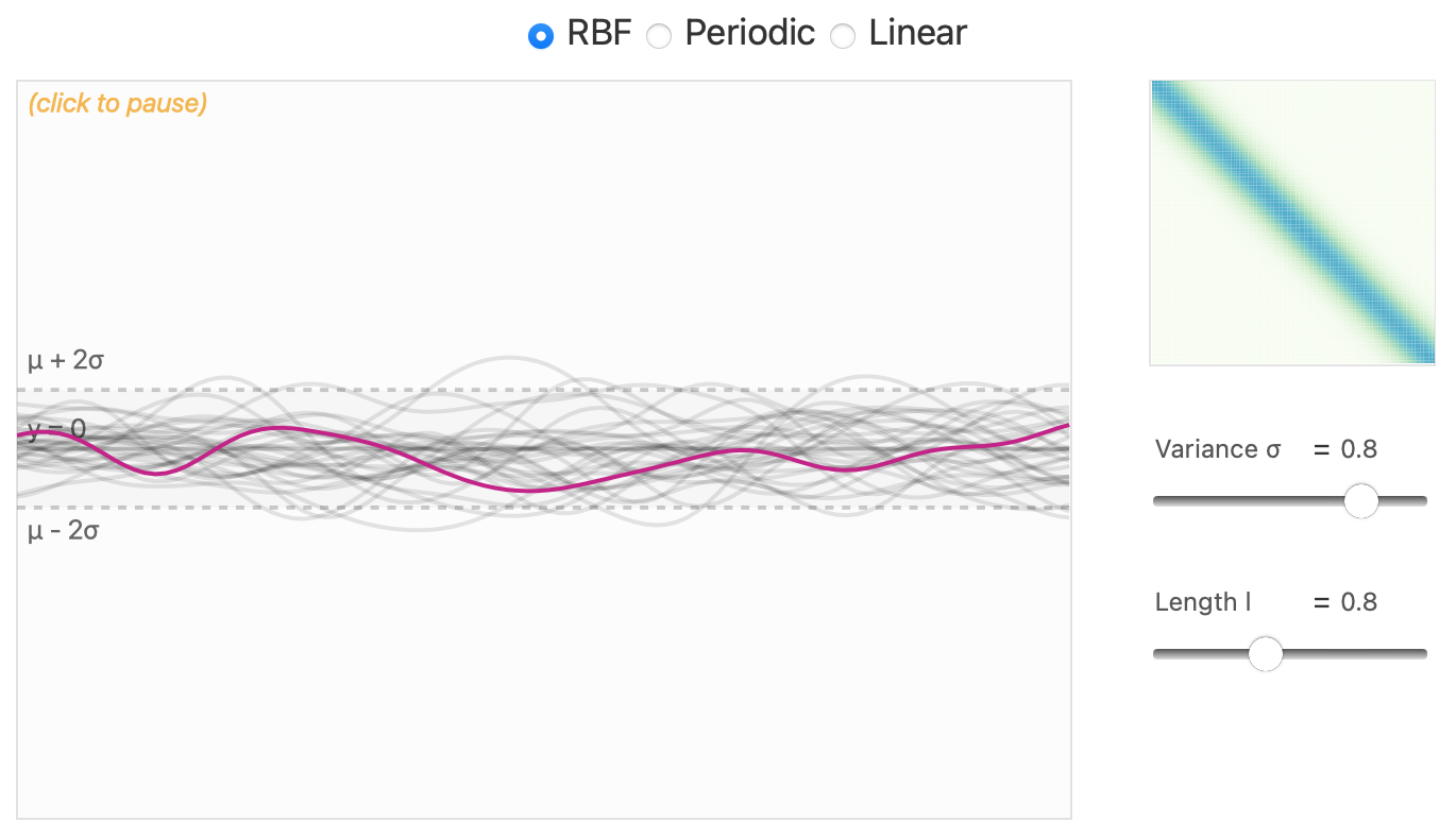
https://distill.pub/2019/visual-exploration-gaussian-processes/
3. Learning Latent Score Function: GP
Periodic Kernel
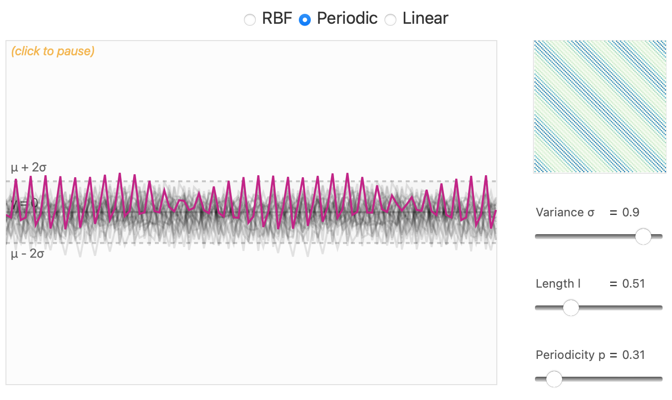
https://distill.pub/2019/visual-exploration-gaussian-processes/
3. Learning Latent Score Function: GP
Linear Kernel
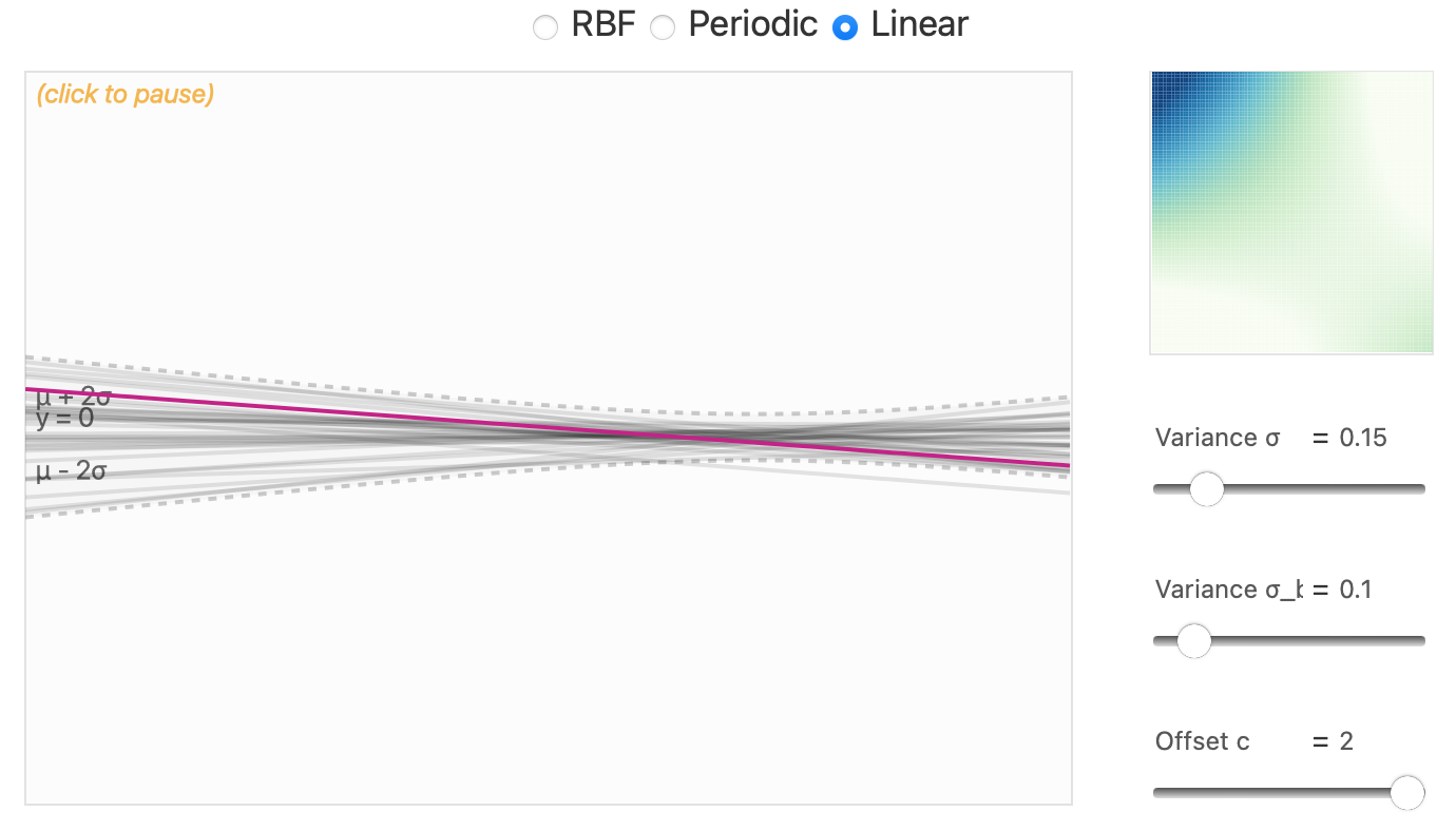
https://distill.pub/2019/visual-exploration-gaussian-processes/
3. Learning Latent Score Function: GP
Analytical Inference: In case the likelihood is Gaussian, the posterior is also Gaussian, and the exact inference can be done as described earlier. For non-Gaussian likelihoods, the posterior is not Gaussian, and exact inference is intractable (i.e., having no closed-form solution).
Numerical Inference: Variational Inference (approximate) or Markov Chain Monte Carlo (asymptotic exact).
3. Learning Latent Score Function: GP
Let us consider a simple example of Gaussian Process binary classification. We have a dataset \(\mathcal{D} = \\{(x_1, y_1), \\dots, (x_N, y_N)\\}\), where \(x_i \in \mathbb{R}^d\) and \(y_i \in \\{-1, +1\\}\). We use Bernoulli distribution to model the data. With a latent function \(f(x)\), the likelihood is given by: \[
p(y_i | x_i) = \sigma(y_i \cdot f(x_i))
\] where \(\sigma(\cdot)\) is the sigmoid function.
3. Learning Latent Score Function: GP
We first present the Elliptical Slice Sampling (ESS) algorithm for sampling from the posterior distribution of the latent function \(f(x)\). - Let the prior distribution of \(f(x)\) be a Gaussian Process with zero mean and covariance matrix \(K\): \(p(f) = \mathcal{N}(f; 0, K)\), where \(K = K(X, X)\). - Step 1: Initializing the latent function \(f^{(0)} \sim \mathcal{N}(0, K)\). - Step 2: Sampling an auxiliary variable \(v \sim \mathcal{N}(0, K)\). - Step 3: Computing likelihood threshold with \(u \sim \mathcal{U}(0, 1)\). \[
\log \pi(f^{(t)}) = \log p(y | f^{(t)}) + \log u
\]
Murray, Adams, and MacKay (2010)
3. Learning Latent Score Function: GP
- Step 3: Drawing a random angle \(\theta \sim \text{Uniform}(0, 2\pi)\), and compute the next latent function: \[
f^{(t+1)} = f^{(t)} \cos(\theta) + v \sin(\theta)
\]
- Step 4: Evaluating the likelihood: \[
\log p(y | f^{(t+1)}) = \sum_{i=1}^N \log \sigma(y_i \cdot f^{(t+1)}(x_i))
\]
- Step 5: If \(\log p(y | f^{(t+1)}) > \log \pi(f^{(t)})\), accept the sample \(f^{(t+1)}\) and return to Step 2. Otherwise, go to Step 6.
Murray, Adams, and MacKay (2010)
3. Learning Latent Score Function: GP
- Step 6: Shrinking the bracket of \(\theta\):
- If \(\theta < 0\), set \(\theta_{\text{min}} = \theta\).
- If \(\theta > 0\), set \(\theta_{\text{max}} = \theta\).
- Step 7: Resampling \(\theta\) from the interval \([\theta_{\text{min}}, \theta_{\text{max}}]\) and return to Step 3.
Murray, Adams, and MacKay (2010)
3. Learning Latent Score Function: GP
- There are multiple methods for approximate inference in Gaussian Processes, such as Laplace Approximation (LA), Expectation Propagation (EP), Variational Bound (VB), or KL-divergence minimization (KL).
- Here is the comparison of some approximate inference methods in posterior approximation:
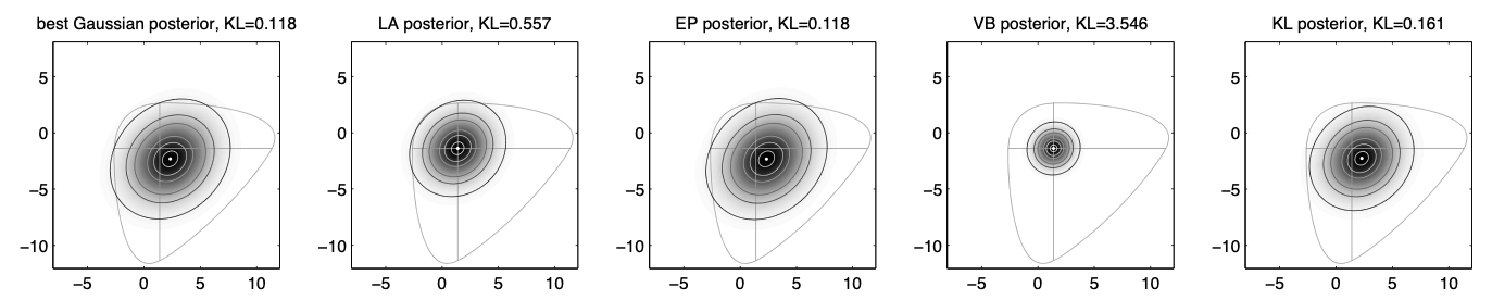
Nickisch and Rasmussen (2008)
3. Learning Latent Score Function: GP
Here is the comparison of some approximate inference methods in likelihood approximation: 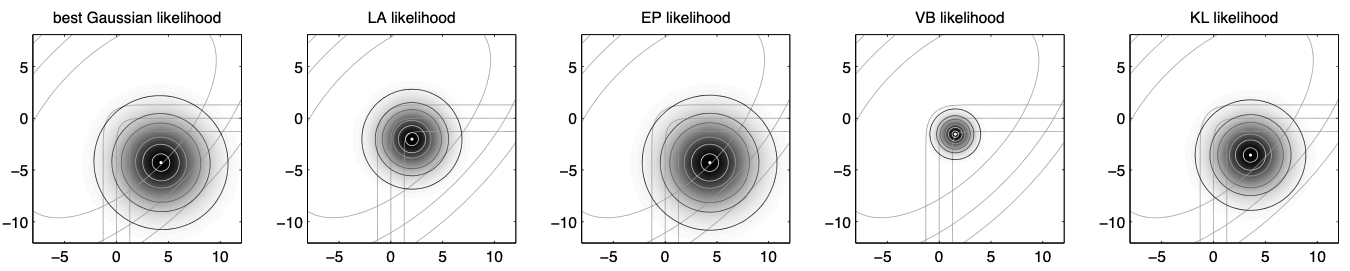
We can observe that the Expectation Propagation (EP) method provides the best approximation for the likelihood.
Nickisch and Rasmussen (2008)
3. Learning Latent Score Function: GP
- Expectation Propagation (EP) is an iterative method to find approximations based on approximate marginal moments.
- The individual likelihood terms are replaced by site functions \(t_i(f_i)\) being unnormalized Gaussians
\[
P(y_i | f_i) \approx t_i(f_i, \mu_i, \sigma_i^2, Z_i) := Z_i\mathcal{N}(f_i | \mu_i, \sigma_i^2)
\] where \(\mu_i\), \(\sigma_i^2\), and \(Z_i\) will be iteratively optimized.
Minka (2013)
3. Learning Latent Score Function: GP
- The posterior approximation is given by: \[
p(f | \mathcal{D}) \approx \mathcal{N}(f | m, (K^{-1} + W)^{-1})
\] where \(W = [\sigma_i^{-2}]_{ii}\) and \(m =[I - K(K + W^{-1})^{-1}]KW\mu\).
- The \(\sigma_i^2\) is an element of the diagonal of the covariance matrix \(K\).
- The \(\mu\) is the mean vector of the Gaussian Process.
Minka (2013); Nickisch and Rasmussen (2008)
3. Learning Latent Score Function: GP
- The likelihood approximation is given by: \[
\begin{aligned}
\log (p(y | x)) &= \log \int p(y | f) p(f | x) df\\
&\approx \log \int \prod_{i=1}^n t_i(f_i, \mu_i, \sigma_i^2, Z_i) p(f | x) df\\
&= \sum_{i=1}^n \log Z_i - \frac{1}{2} \mu^{\top}(K + W^{-1})^{-1} \mu\\
&- \frac{1}{2}\log |K+W^{-1}| - \frac{n}{2}\log 2\pi
\end{aligned}
\] Minka (2013); Nickisch and Rasmussen (2008)
4. Policy for PBO
In practice, the new duels are queried sequentially. Thus, it may be very expensive if we do not have a good acquisition strategy, as we need to explore a lot of duels before finding the Condorcet winner.
To address this issue, we can formulate this problem as an active preference learning problem, where we can customize the acquisition function to balance between exploration and exploitation, helping to find the Condorcet winner with fewer duels.
4. Policy for PBO
In this lecture, we will explore three acquisition functions which can be used to find the Condorcet winner: - Pure exploration - Copeland Expected Improvement - Dueling-Thompson sampling
González et al. (2017)
4. Policy for PBO
Pure Exploration - The goal of pure exploration is to find the duel of which the preference score is the most uncertain (highest variance). - We can qualify the uncertainty of the preference score by computing the variance of it: \[
\begin{aligned}
\mathcal{V}[\sigma(f_t) | [x_t, x_t'] | \mathcal{D}, \theta] &= \int \left( \sigma(f_t) - \mathbb{E}\left[ \sigma(f_t) \right] \right)^2 p(f_t | \mathcal{D}, [x_t, x_t'], \theta) df_t\\
&= \int \sigma(f_t)^2 p(f_t | \mathcal{D}, [x_t, x_t'], \theta) df_t - \mathbb{E}\left[ \sigma(f_t) \right]^2
\end{aligned}
\]
In practice, we can approximate the variance by using Monte-Carlo sampling.
González et al. (2017)
4. Policy for PBO
Copeland Expected Improvement - The idea of Expected Improvement is to find the duels that have a higher preference score than the current best one. - We denote \(c_{x}^* = C(x; \mathcal{D}_t, \theta)\) is the estimated Condorcet winner resulting from \(\mathcal{D}_t = \mathcal{D} \cup \\{[x_t,x_t'],1\\}\). - We also denote \(c_{x'}^* = C(x'; \mathcal{D}_t, \theta)\) is the estimated Condorcet winner resulting from \(\mathcal{D}_t = \mathcal{D} \cup \\{[x_t,x_t'],0\\}\). - The Copeland Expected Improvement is defined as: \[
\begin{aligned}
A_{\text{CEI}}([x_t, x_t'] | \mathcal{D}, \theta) &= \pi([x, x']|\mathcal{D}_t, \theta)(c^*_{x} - c^*)\\
&+ \pi([x', x]|\mathcal{D}_t, \theta)(c^*_{x'} - c^*)
\end{aligned}
\]
González et al. (2017)
4. Policy for PBO
Dueling-Thompson Sampling - The above two acquisition functions have some limitations: - Pure exploration is too explorative and does not exploit the knowledge about the current best location. - Copeland Expected Improvement is over-exploitative and expensive to compute. - Thompson sampling can be used to balance between exploration and exploitation. The idea is to sample the preference score from the posterior distribution and select the duel with the highest preference score.
González et al. (2017)
4. Policy for PBO
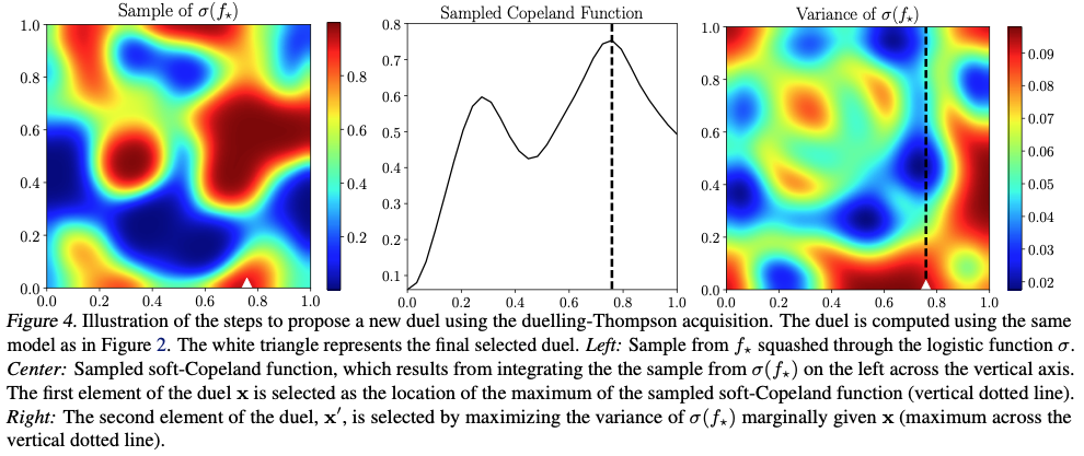
Dueling-Thompson Sampling
Step 1 (Selecting \(x_t\)): At first, we sample an \(\tilde{f}\) from the model using continuous Thompson sampling and compute the soft Copeland score as: \[
x_{t} = \arg \max_{x \in \mathcal{X}} \int_{\mathcal{X}} \pi_{\tilde{f}}([x, x']; \mathcal{D}, \theta) dx'
\] where \(\pi_{\tilde{f}}([x_t, x_t'];\mathcal{D}, \theta) = \int \sigma(\tilde{f}_t) p(\tilde{f}_t | \mathcal{D}, [x_t, x_t'], \theta) d\tilde{f}_t\).
González et al. (2017)
4. Policy for PBO
Dueling-Thompson Sampling
Step 2 (Selecting \(x'\)): Given \(x_t\), the \(x_t'\) is selected to maximize the variance of \(\sigma(f_t)\) in the direction of \(x_t\): \[
x'_{t} = \arg \max_{x'_t \in \mathcal{X}} \mathcal{V}[\sigma(f_t) | [x_t, x_t'] | \mathcal{D}, \theta]
\]
Finally, the selected duel \([x_t, x_t']\) is queried, and the process is repeated until the Condorcet winner is found.
González et al. (2017)
4. Policy for PBO
Dueling-Thompson Sampling
González et al. (2017)
4. Policy for PBO
Dueling-Thompson Sampling
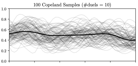
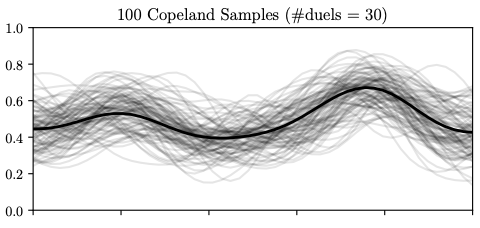
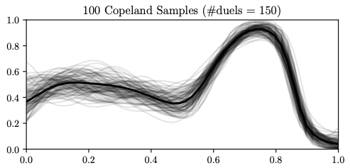
100 continuous samples of the Copeland score function (grey) in the Forrester example were generated using Thompson sampling. The three plots show the samples obtained once the model has been trained with different numbers of duels (10, 30, and 150). In black, we show the Copeland function computed using the preference function. The more samples are available, more exploitation is encouraged in the first element of the duel as the probability of selecting \(x_t\) as the true optimum increases.
González et al. (2017)
5. Decision-Theoretic Acquisition Function
We restart with a more general problem where we have a set of more-than-2 points to get the preference feedback. - Let us denote \(X = (x_1, \dots, x_q) \in \mathcal{X}^q\) is a query containing \(q\) points and \(g(\cdot)\) is the latent function. - Starting with the one-step Bayes optimal policy, we define the expected utility received after querying \(X \in \mathcal{X}^q\) as: \[
V_t(X) = \mathbb{E}_t \left[ \max_{x \in \mathcal{X}} \mathbb{E}_{t+1} [g(x)] | X_{t+1} = X \right]
\]
Astudillo et al. (2023)
5. Decision-Theoretic Acquisition Function
The goal is to find \(X\) that maximizes the expected utility \(V_t(X)\). \[
X_t = \arg \max_{X \in \mathcal{X}^q} V_t(X)
\]
Since \(\max_{x \in \mathcal{X}} \mathbb{E}_{t+1} [g(x)]\) is not dependent on \(X_t\), we can rewrite the expected utility as: \[
\begin{aligned}
V_t(X) &= \mathbb{E}_t \left[ \max_{x \in \mathcal{X}} \mathbb{E}_{t+1} [g(x)] | X_{t+1} = X \right]\\
&\propto \mathbb{E}_t \left[ \max_{x \in \mathcal{X}} \mathbb{E}_{t+1} [g(x)] - \max_{x \in \mathcal{X}} \mathbb{E}_{t} [g(x)] \vert X_{t+1} = X \right]\\
\end{aligned}
\] Astudillo et al. (2023)
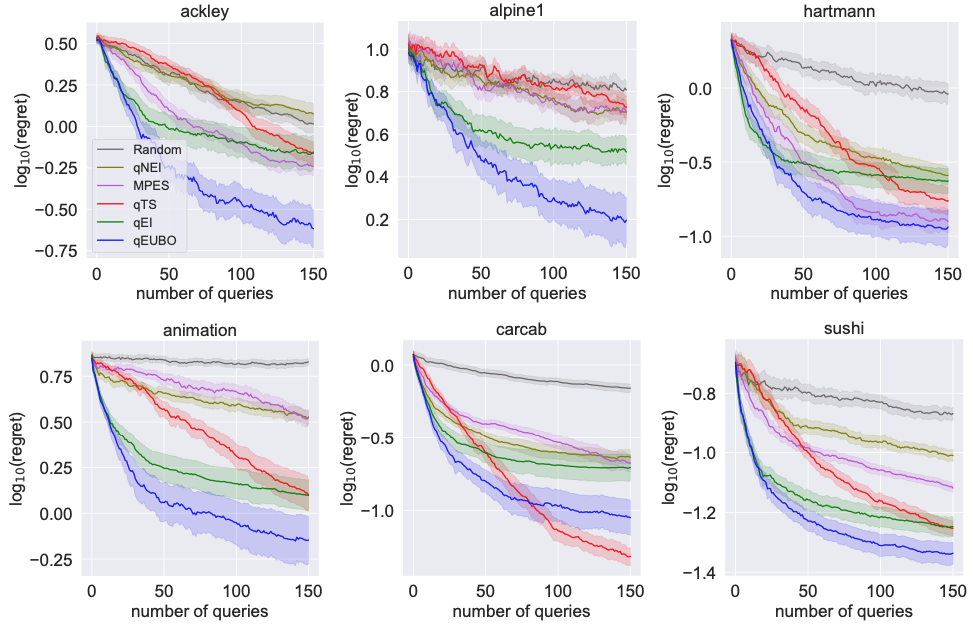
5. Decision-Theoretic Acquisition Function
We define the expected utility of the best option (qEUBO) as: \[
A_{qEUBO, t} (X) = \mathbb{E} \left[ \{ g(x_1), \dots, g(x_q) \} \right]
\] According to Theorem 1 in (Astudillo et al., 2023), we have: \[
\arg \max_{X \in \mathcal{X}^q} A_{qEUBO, t} (X) \subseteq \arg \max_{X \in \mathcal{X}^q} V_t(X)
\] Thus, optimizing the expected utility of the query is sufficient to find the optimal query (i.e., maximize the \(A_{qEUBO, t}\)).
Astudillo et al. (2023)
5. Decision-Theoretic Acquisition Function
Theorem 1: - Suppose the actor responses are noise-free. - Then \[\arg \max_{X \in \mathcal{X}^q} A_{qEUBO, t} (X) \subseteq \arg \max_{X \in \mathcal{X}^q} V_t(X)\]
Proof Outline: 1. For each \(X \in \mathcal{X}\) and \(i \in \{1, \ldots, q\}\), define \(X^+(X) = \{x^+(X, i)\}\), where \(x^+(X, i) = \arg \max_{x \in \mathcal{X}} \mathbb{E}_t[g(x) \mid (X, i)]\). 2. Show that: \[V_t(X) \leq A_{qEUBO, t}(X^+(X))\]
5. Decision-Theoretic Acquisition Function
Proof of Theorem 1
For any given \(X \in \mathcal{X}\) and each \(i \in \{1, \dots, q\}\),
let \(x^+(X, i) \in \arg \max_{x \in \mathcal{X}} \mathbb{E}_t[g(x) \mid (X, i)]\),
and define \(X^+(X) = (x^+(X, 1), \dots, x^+(X, q))\).
We claim that: \[
V_t(X) \leq A_{qEUBO, t}(X^+(X))
\]
5. Decision-Theoretic Acquisition Function
Proof of Theorem 1
To see this, we denote \(r(X) \in \{1, \dots, q\}\) as the index of the component of \(X^+(X)\) that maximizes the expected utility of the best option: \[
V_t(X) = \sum_{i=1}^{q} P_t(r(X) = i) \mathbb{E}_t[g(x^+(X, i)) | (X, i)]
\] \[
\leq \sum_{i=1}^{q} P_t(r(X) = i) \mathbb{E}_t\left[\max_{i=1,\dots,q} g(x^+(X, i)) \mid (X, i)\right]
\] \[
= \mathbb{E}_t\left[\max_{i=1,\dots,q} g(x^+(X, i))\right]
= A_{qEUBO, t}(X^+(X))
\]
5. Decision-Theoretic Acquisition Function
Proof of Theorem 1
On the other hand, for any given \(X \in \mathcal{X}^q\), we have: \[
\mathbb{E}_t[g(x_{r(X)}) | (X, r(X))] \leq \max_{x \in \mathcal{X}} \mathbb{E}_t[g(x) | (X, r(X))].
\] Since \(g(x_{r(X)}) = \max_{i=1,\dots,q} g(x_i)\), taking expectations over \(r(X)\) on both sides, we obtain: \[
A_{qEUBO, t}(X) \leq V_t(X).
\]
5. Decision-Theoretic Acquisition Function
Proof of Theorem 1
Now, building on the arguments above, let \(X^* \in \arg \max_{X \in \mathcal{X}} A_{qEUBO, t}(X)\) and suppose for the sake of contradiction that \(X^* \notin \arg \max_{X \in \mathcal{X}} V_t(X)\).
Then, there exists \(\tilde{X} \in \mathcal{X}^q\) such that \(V_t(\tilde{X}) > V_t(X^*)\). By the arguments above, we have: \[
A_{qEUBO, t}(X^+(\tilde{X})) \geq V_t(\tilde{X}) > V_t(X^*) \geq A_{qEUBO, t}(X^*(X)),
\] which contradicts the assumption. Therefore, the claim holds.
5. Decision-Theoretic Acquisition Function
Proof of Theorem 1
The first inequality follows from \((1)\). The second inequality is due to our supposition for contradiction. The third inequality is due to \((2)\). Finally, the fourth inequality holds since \(X^* \in \arg \max_{X \in \mathcal{X}} A_{qEUBO, t}(X)\).
This contradiction concludes the proof.
5. Decision-Theoretic Acquisition Function
In case there are noises in the actor responses, maximizing \(A_{qEUBO, t}\) is not equivalent to maximizing \(V_t\).
However, if the noises in responses follow the logistic likelihood function \(L(g(x); \lambda)\) with noise level parameter \(\lambda\), \(qEUBO\) can still be highly effective. Each component in \(L(g(x); \lambda)\) is a logistic function defined as follows. \[
L_i(g(x); \lambda) = \frac{\exp (g(x_i) / \lambda)}{\sum_{j=1}^q \exp (g(x_j) / \lambda)}
\]
5. Decision-Theoretic Acquisition Function
We denote \(V\_t\) as \(V\_t^\lambda\) to make its dependence on \(\lambda\) explicit. If \(X^* \in \arg \max_{X \in \mathcal{X}} A_{qEUBO, t}(X)\), then we have Theorem 2 as: \[
V_t^{\lambda}(X^*) \geq \max_{X \in \mathcal{X}} V_t^0(X) - \lambda C,
\] where \(C = L_W((q - 1)/ e)\), and \(L_W\) is the Lambert W function (Corless et al., 1996).
Corless et al. (1996)
5. Decision-Theoretic Acquisition Function
Lemma 1: For any \(s_1, \dots, s_q \in \mathbb{R}\), \[
\sum_{i=1}^q \frac{\exp(s_i/\lambda)}{\sum_{j=1}^q \exp(s_j/\lambda)} s_i \geq \max_{i=1,\dots,q} s_i - \lambda C,
\] where \(C = L_W((q - 1)/ e)\), where \(L_W\) is the Lambert W function (Corless et al., 1996).
Corless et al. (1996); Astudillo et al. (2023)
5. Decision-Theoretic Acquisition Function
Proof of Lemma 1
We may assume without loss of generality that \(\max_{i=1,\dots,q} s_i = s_q\). Let \(t_i = (s_q - s_i)/\lambda\) for \(i \in \{1,\dots,q-1\}\). After some algebra, we see that the inequality we want to show is equivalent to \[
\sum_{i=1}^{q-1} \frac{t_i \exp(-t_i)}{1 + \sum_{j=1}^{q-1} \exp(-t_j)} \leq C.
\]
Astudillo et al. (2023)
5. Decision-Theoretic Acquisition Function
Proof of Lemma 1 (cont)
Thus, it suffices to show that the function \(\eta : [0,\infty)^{q-1} \to \mathbb{R}\) given by \[
\eta(t_1, \dots, t_{q-1}) = \sum_{i=1}^{q-1} \frac{t_i \exp(-t_i)}{1 + \sum_{j=1}^{q-1} \exp(-t_j)}
\] is bounded above by \(C\).
Viappiani and Boutilier (2010); Astudillo et al. (2023)
5. Decision-Theoretic Acquisition Function
Lemma 2: \(\mathbb{E}\_t^{\lambda} [g(x_{r(X)})] \geq A\_{qEUBO, t}(X) - \lambda C\) for all \(X \in \mathcal{X}\). Note that \[
\mathbb{E}_t^{\lambda}[g(x_{r(X)}) | g(x)] = \sum_{i=1}^q \frac{\exp(g(x_i)/\lambda)}{\sum_{j=1}^q \exp(g(x_j)/\lambda)} g(x_i).
\] Lemma 1 implies \[\mathbb{E}_t^{\lambda}[g(x_{r(X)}) | g(x)] \geq \max_{i=1:q} g(x_i) - \lambda C.\] Taking expectations over both sides yields the conclusion.
5. Decision-Theoretic Acquisition Function
Lemma 3: \(V_t^{\lambda}(X) \geq \mathbb{E}\_t^{\lambda} [g(x_{r(X)})]\) for all \(X \in \mathcal{X}\).
Observe that \[
\begin{aligned}
V_t^{\lambda}(X) &= E_t^{\lambda}\left[\max_{x \in \mathcal{X}} E[g(x) | (X, r(X))]\right]\\
&\geq E_t^{\lambda}[E[g(x_{r(X)}) | (X, r(X))]]\\
&= E_t^{\lambda}[g(x_{r(X)})]
\end{aligned}
\] where the penultimate equality is followed by the law of iterated expectation.
5. Decision-Theoretic Acquisition Function
Recall the Theorem 2, if we have \(X^* \in \arg \max_{X\in \mathcal{X}^q} A_{qEUBO, t}(X)\), then: \[
V_t^{\lambda}(X^*) \geq \max_{X \in \mathcal{X}^q} V_t^0(X) - \lambda C
\]
Let \(X^{**} \in \arg \max_{X \in \mathcal{X}^q} V_t^0(X)\). We have the following chain of inequalities:
\[
\begin{aligned}
V_t^{\lambda}(X^{*}) &\geq \mathbb{E}_t^{\lambda} [g(x_{r(X^*)})]\\
&\geq \mathbb{E}_t^{0} [g(x_{r(X^*)})] - \lambda C\\
&= A_{qEUBO, t}(X^{*}) - \lambda C \geq A_{qEUBO, t}(X^{**}) - \lambda C\\
&\geq V_t^0(X^{**}) - \lambda C = \max_{X \in \mathcal{X}} V_t^0(X) - \lambda C.
\end{aligned}
\]
5. Decision-Theoretic Acquisition Function
- The first inequality follows from Lemma 3.
- The second inequality follows from Lemma 2.
- The third line (first equality) follows from the definition of \(A_{qEUBO, t}\).
- The fourth line (third inequality) follows from the definition of \(X^{*}\).
- The fifth line (fourth inequality) can be obtained as in the proof of Theorem 1.
- Finally, the last line (second equality) follows from the definition of \(X^{**}\).
5. Decision-Theoretic Acquisition Function
Astudillo et al. (2023)
Summary
- In this lecture, we have learned about Preferential Bayesian Optimization, a method for optimizing black-box functions using preference feedback.
- We have discussed the Gaussian Process regression, which is used to model the underlying distribution of the function.
- We have also explored different acquisition functions, including Pure Exploration, Copeland Expected Improvement, and Dueling-Thompson Sampling, to find the Condorcet winner.
- Finally, we have introduced the qEUBO, which aims to maximize the expected utility of the query.