Machine Learning from Human Preferences
Chapter 4: Dueling Bandits
1. Introduction to Dueling Bandit
Motivation
- In real-world applications, the reward of each action is not directly observable. Instead, the reward of each action is observed through a comparison with another action(s).
- Example: In a movie recommendation system, the reward of each movie is not directly observable. Instead, the reward is observed through the comparison of two or more movies.


Which one do you prefer?
1. Introduction to Dueling Bandit
Motivation
- Theoretically, we can model this setting as a dueling bandit problem, where the reward of each action is observed through a comparison with another action(s).
- There are two main types of dueling bandit problems: contextual dueling bandit and non-contextual dueling bandit.
- The contextual dueling bandit problem is a variant of the dueling bandit problem where the decision-maker has access to the context which can help to make a better decision.
1. Introduction to Dueling Bandit
Multi-Armed Bandit Problem
- The multi-armed bandit problem is a classical problem in sequential decision making. This problem involves a player at a row of slot machines who has to decide which machines to play, how many times to play each machine, and in which order to play them.
- The objective is to maximize the player’s total reward over a sequence of plays.

1. Introduction to Dueling Bandit
Dueling Bandit Problem
- The dueling bandit problem is a variant of the multi-armed bandit problem where the reward of each turn is not observed directly. Instead, the player observes the pairwise comparison of the rewards of two arms.
- The objective is to find the best arm without knowing the reward of each arm after each play.
1. Introduction to Dueling Bandit
- Let’s define the dueling bandit problem formally. Consider a set of \(K\) bandits \(\mathcal{B} = \{ b_1, \dots, b_K\}\).
- At each round \(t\), the player selects a pair of bandits \(b_i, b_j \in \mathcal{B}\) and observes the comparison \(c_{ij} \in \{1, -1\}\), where \(c_{ij} = 1\) if \(b_i\) is preferred to \(b_j\) and \(c_{ij} = -1\) otherwise.
1. Introduction to Dueling Bandit
- Recall the Bradley-Terry model, which models the probability of \(b_i\) being preferred to \(b_j\) as \(P(b_i \succ b_j ) \in (0,1)\), we can define the model in this setting as:
\[ P(b_i \succ b_j) = (c_{ij} + 1) / 2 \] - Let us denote \(\epsilon(b_i, b_j) = c_{ij} / 2\). We can rewrite the Bradley-Terry model as follows:
\[ P(b_i \succ b_j) = \epsilon(b_i, b_j) + \frac{1}{2} \]
1. Introduction to Dueling Bandit
By this model, we have the following properties: \[ \epsilon(b_i, b_i) = 0, \epsilon(b_i, b_j) = -\epsilon(b_j, b_i)\text{ and,} \] \[ b_i \succ b_j \text{ if and only if } \epsilon(b_i, b_j) > 0 \] We also assume there is a total order over the bandits, i.e., there exists a permutation \(\varphi\) such that \(b_{\varphi(1)} \succ b_{\varphi(2)} \succ \dots \succ b_{\varphi(K)}. Without loss of generality, we have\)$ b_i b_j (i) < (j) $$ Thus, the best bandit is \(b_{\varphi(1)}\).
1. Introduction to Dueling Bandit
To qualify the decision at each turn \(t\), we start to construct the regret measurement. Recall that the probability of winning or losing in a pairwise comparison is at least \(0.5\), the instantaneous regret is defined as: \[ r_t = P(b_{\varphi(1)} \succ b_1) + P(b_{\varphi(1)} \succ b_2) - 1 \] where \(r_t\) is the regret of the decision at turn \(t\).
1. Introduction to Dueling Bandit
Then, the total cumulative regret is defined as: \[ \begin{aligned} R_T = \sum_{t=1}^{T} r_t &= \sum_{t=1}^{T} \left[ P(b_{\varphi(1)} \succ b_{1,t}) + P(b_{\varphi(1)} \succ b_{2,t}) - 1 \right]\\ &= \sum_{t=1}^{T} \left[\left(\epsilon(b_{\varphi(1)}, b_{1,t}) + \frac{1}{2}\right) + \left(\epsilon(b_{\varphi(1)}, b_{2,t}) + \frac{1}{2}\right) - 1\right]\\ &= \sum_{t=1}^{T} \left[\epsilon(b_{\varphi(1)}, b_{1,t}) + \epsilon(b_{\varphi(1)}, b_{2,t})\right] \end{aligned} \] where \(R_T\) is the total cummulative regret after \(T\) turns.
2. Contextual Dueling Bandit
- In real-world applications, many problems require the decision-maker to have access to the context to make a better decision.
- For example, in a movie recommendation system, the context can be the user’s age, gender, the movie’s genre, release year, etc.
- Formally, we assume that at each round \(t\), the player observes a context \(x_t \in \mathcal{X}\), where \(\mathcal{X}\) is the context space.
- Thus, we can model the output of the dueling bandit problem as a function of the context and the bandits, i.e., \(\epsilon: \mathcal{X} \times \mathcal{B} \rightarrow \mathcal{Y}\).
\[ \epsilon(b_i, b_j | x_i, x_j) \in \left[\frac{-1}{2}, \frac{1}{2}\right] \]
2. Preference Learning for Dueling Bandit
- The goal of preference active learning is to find the best bandit \(b_{\varphi(1)}\) with the minimum number of turns (i.e., minimum number of pulled bandits).
- In this problem, the preference learning method must take both exploration and exploitation into account.
2. Preference Learning for Dueling Bandit
Traditional acquisition functions for dueling bandit problem: - Interleaved Filtered (Yue et al., 2012) - Thompson Sampling (Agrawal & Goyal, 2013) - Dueling Bandit Gradient Descent (DBGD) (Dudík et al., 2015)
Auer (2002); Yue et al. (2012); Agrawal and Goyal (2013); Dudik et al. (2015)
3. Dueling Posterior Sampling
- Dueling Posterior Sampling (DPS) is a Bayesian method for solving the contextual dueling bandit problem.
- It employs preference-based posterior sampling to learn both the system dynamics and the underlying utility function that governs the preference feedback.
- In this method, we consider a fixed-horizon Markov Decision Process (MDP) with a finite number of states and actions.
- We denote the state space as \(\mathcal{S}\) and the action space as \(\mathcal{A}\).
- We can observe that, in this setting, the context \(x_t\) can be defined by the states \(s_t\), and the bandits \(b_i, b_j\) are the actions \(a_i, a_j\).
- In this lecture, we consider the discrete state space and action space.
Novoseller et al. (2020)
3. Dueling Posterior Sampling
- At each turn \(t\), the player selects a pair of actions \(a_i, a_j \in \mathcal{A}\).
- We denote the length-\(h\) trajectory of the agent as \(\tau = (s_1, a_1 s_2, a_2, \dots, s_h, a_h, s_{h+1})\).
- In the \(i^{th}\) round, the agent rolls out the trajectory \(\tau_{i1}\), \(\tau_{i2}\), and observes the preference feedback.
- We denote the transition probability as \(p(s_{t+1} | s_t, a_t)\) and the preference function \(\phi\) as \(\phi(\tau_{1}, \tau_{2}) = P(\tau_{1} \succ \tau_{2})\).
Novoseller et al. (2020)
3. Dueling Posterior Sampling
- We introduce the policy \(\pi: \mathcal{S} \times \{1,\dots,h\} \to \mathcal{A}\) that maps the state \(s_t\) to the action \(a_t\).
- At each iteration \(i\), the agent samples two policies \(\pi_{i1}\), \(\pi_{i2}\). The agent then samples the trajectories \(\tau_{i1}\), \(\tau_{i2}\) using the policies \(\pi_{i1}\), \(\pi_{i2}\), respectively.
- With a policy \(\pi\), we can compute the expected utility of the trajectory \(\tau\) (i.e., value function) starting at step \(j\) as: \[ V_{\pi, j}(s) = \mathbb{E}_{\pi} \left[ \sum_{t=j}^{h} \bar{r}(s_t, \pi(s_t, t)) | s_j = s \right] \] where \(\bar{r}(s_t, a_t)\) is the expected utility of the action \(a_t\) at state \(s_t\).
Novoseller et al. (2020)
3. Dueling Posterior Sampling
- Our goal is to find optimal policy \(\pi^*\) which can maximize the expected utility of all input states. \[ \pi^* = \arg \sup_{\pi} \sum_{s\in\mathcal{S}} p_0(s)V_{\pi, 1}(s) \] where \(p_0(s)\) is the initial state distribution.
Novoseller et al. (2020)
3. Dueling Posterior Sampling
- We quantify the learning agent performance via its cumulative T-step Bayesian regret relative to the optimal policy \[ \mathbb{E}[\text{Reg}(T)] = \mathbb{E} \left\{ \sum_{i=1}^{\left\lceil \frac{T}{2h} \right\rceil} \sum_{s \in \mathcal{S}} p_0(s) \left[ 2V_{\pi^*,1}(s) - V_{\pi_{i1},1}(s) - V_{\pi_{i2},1}(s) \right] \right\}. \]
Novoseller et al. (2020)
3. Dueling Posterior Sampling
The DPS algorithm is summarized as follows:
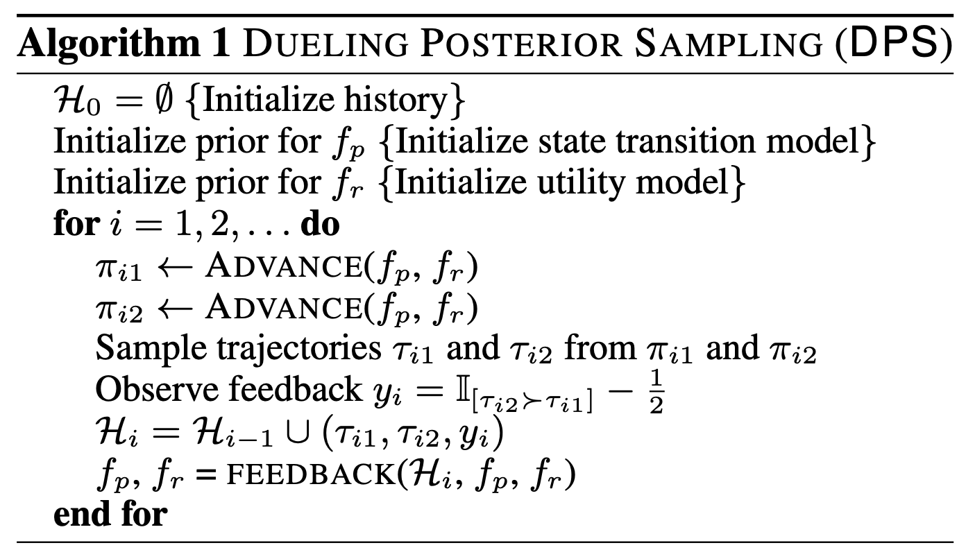
where \(\mathbb{I}_{[\tau_{i2} \succ \tau_{i1}]} = P(\tau_{i2} \succ \tau_{i1})\) is the indicator function that returns \(1\) if \(\tau_{i2} \succ \tau_{i1}\) and \(0\) otherwise.
Novoseller et al. (2020)
3. Dueling Posterior Sampling
ADVANTAGE: Sample policy from dynamics and utility models
Input: \(f_p\): state transition posterior, \(f_r\): utility posterior 1. Sample \(\tilde{p} \sim f_p(\cdot)\) 2. Sample \(\tilde{r} \sim f_r(\cdot)\) 3. Solve \(\pi^* = \arg \sup_{\pi} \sum_{s\in\mathcal{S}} p_0(s)V_{\pi, 1}(s | \tilde{p}, \tilde{r})\) 4. Return \(\pi^*\)
Novoseller et al. (2020)
3. Dueling Posterior Sampling
FEEDBACK: Update dynamics and utility models based on new user feedback
Input: \(\mathcal{H} = \{ \tau_{i1}, \tau_{i2}, y_i \}\), \(f_p\): state transition posterior, \(f_r\): utility posterior 1. Apply Bayesian update to \(f_p\) using \(\mathcal{H}\) 2. Apply Bayesian update to \(f_r\) using \(\mathcal{H}\) 3. Return \(f_p\), \(f_r\)
Novoseller et al. (2020)
3. Dueling Posterior Sampling
In DPS, the process of updating the dynamics posterior is straightforward. We can assume the dynamics are fully observed and model them with Dirichlet distribution. Then, the likelihood of the state transition is multinomial, and we can update the posterior as follows: \[ f_p(s_{t+1} | s_t, a_t) = \text{Dirichlet}(\alpha + \text{count}(s_{t+1} | s_t, a_t)) \]
This formula can be interpreted as we update the posterior by adding the count of the new state to the prior.
3. Dueling Posterior Sampling
- The utility posterior is more complex because we perform Bayesian inference over state-action pairs, and feedback is at trajectory level.
- Based on Novoseller et al. (2020), we can model the utility using Bayesian linear regression.
Novoseller et al. (2020)
3. Dueling Posterior Sampling
Theoretical Analysis
We will now analyze the asymptotic Bayesian regret of DFS under a Bayesian linear regression model. The analysis contains three steps: 1. Proving DPS is asymptotic-consistent (i.e., the probability of selecting the optimal policy converges to 1). 2. Bounding one-sided Bayesian regret for \(\pi_{i2}\), which means DPS is only able to select \(\pi_{i2}\) and \(\pi_{i1}\) is sampled from a fixed distribution. 3. Assuming the distribution of \(\pi_{i1}\) is drifting but converging, we bound the Bayesian regret for \(\pi_{i2}\).
Novoseller et al. (2020)
3. Dueling Posterior Sampling
Asymptotic consistency of DPS
- Prior to proving the asymptotic consistency of DPS, we need to prove that the posterior distribution of the dynamics and utility models converge to the true distribution.
Proposition 1: The sampled dynamics converge in distribution to their true value as the DPS iteration increase 1. Let the posterior distribution of the dynamics for each state-action pair \(s_t, a_t\) be \(P(s_{t+1} | s_t, a_t)\) and the true distribution be \(P^*(s_{t+1} | s_t, a_t)\), with \(\epsilon > 0\) and \(\delta > 0\): \[ P(|P(s_{t+1} | s_t, a_t) - P^*(s_{t+1} | s_t, a_t)| > \epsilon) < \delta \]
3. Dueling Posterior Sampling
Asymptotic consistency of DPS
Let \(N(s, a)\) represent the number of times state-action pair \(s, a\) has been observed. As \(N(s, a) \to \infty\), the posterior distribution concentrates around the true distribution \(P^*(s_{t+1} | s_t, a_t)\).
The remaining problem is to prove that DPS will visit all state-action pairs infinitely often.
Novoseller et al. (2020)
3. Dueling Posterior Sampling
Asymptotic consistency of DPS
Lemma 3 (Novoseller et al., 2020): Under DPS, every state-action pair is visited infinitely-often.
Proof sketch: - The proof proceeds by assuming that there exists a state-action pair that is visited only finitely-many times. - This assumption will lead to a contradiction: once this state-action pair is no longer visited, the reward model posterior is no longer updated with respect to it. Then, DPS is guaranteed to eventually sample a high enough reward for this state-action that the resultant policy will prioritize visiting it.
Novoseller et al. (2020)
3. Dueling Posterior Sampling
Asymptotic consistency of DPS
Proposition 2: With probability of \(1 - \delta\), where delta is a parameter of the Bayesian linear regression model, the sampled rewards converge in distribution to the true reward parameters, \(\bar{r}\), as the DPS iteration increases.
Novoseller et al. (2020)
3. Dueling Posterior Sampling
Asymptotic consistency of DPS
According to Theorem 2 from Abbasi-Yadkori et al. (2011), under certain regularity conditions, we can bound the error between the estimated reward parameter \(\hat{r}_i\) and the true reward parameter \(r_i\) with high probability. With probability at least \(1 - \delta\): \[ \| \hat{r}_i - r_i \|_{\mathbf{M}_i} \leq \beta_i(\delta) \] - \(\mathbf{M}_i\): design (covariance) matrix - \(\beta_i(\delta)\): confidence bound (depends on \(\delta\)) - This defines an ellipsoid around the true reward parameters.
Novoseller et al. (2020)
3. Dueling Posterior Sampling
Asymptotic consistency of DPS
- The posterior covariance matrix \(\mathbf{M}_i^{-1}\) shrinks with more observations.
- Eigenvalues \(\lambda_{i,j}\) of the covariance matrix tend to zero: \[ \lim_{i \to \infty} \lambda_{i,j} \to 0 \]
- This implies uncertainty in the reward parameters decreases over time, which implies the reward parameters converge to the true values.
Novoseller et al. (2020)
3. Dueling Posterior Sampling
Asymptotic consistency of DPS
Theorem 1: With probability \(1 - \delta\), the sampled policies \(\pi_{i1}, \pi_{i2}\) converge in distribution to the optimal policy \(\pi^*\) as \(i \to \infty\).
- From Propositions 1 and 2, \(\tilde{p}_{i1} \overset{D}{\to} p\) and \(\tilde{r}_{i1} \overset{D}{\to} r\) (with probability \(1 - \delta\))
- The reward function \(\tilde{r}_{i1}\) converges in distribution to the true reward parameters \(r\).
- For each fixed \(\pi\), the value function \(V(\tilde{p}_{i1}, \tilde{r}_{i1}, \pi)\) converges in distribution to \(V(p, r, \pi)\) as value functions are continuous in the dynamics and reward parameters.
Novoseller et al. (2020)
3. Dueling Posterior Sampling
Asymptotic consistency of DPS
- Applying Fact 2 (Appendix A.5) in Novoseller et al. (2020), we have: \[ P\left( \left| V(\tilde{p}_{i1}, \tilde{r}_{i1}, \pi) - V(p, r, \pi) \right| > \epsilon \right) \to 0 \quad \text{as} \quad i \to \infty \] This shows that the value of the sampled policies converges to that of the optimal policy.
Novoseller et al. (2020)
3. Dueling Posterior Sampling
Bound the one-sided regret under a fixed \(\pi_{i1}\)-distribution
- We adapt information-theoretic analysis from Russo and Van Roy (2016) to incooperate preference feedback and state-transition dynamics.
- The trade-off between exploration and exploitation is defined as: \[ \Gamma_i = \frac{ \mathbb{E}_i[ (y^*_i - y_i)^2 ] }{ \mathbb{I}_i[\pi^*; (\pi_{i2}, \tau_{i1}, \tau_{i2}, x_{i2} - x_{i1}, y_i )] } \]
Russo and Van Roy (2016); Novoseller et al. (2020)
3. Dueling Posterior Sampling
Bound the one-sided regret under a fixed \(\pi_{i1}\)-distribution
\[ \Gamma_i = \frac{ \mathbb{E}_i[ (y^*_i - y_i)^2 ] }{ \mathbb{I}_i[\pi^*; (\pi_{i2}, \tau_{i1}, \tau_{i2}, x_{i2} - x_{i1}, y_i )] } \] - Numerator: Squared instantaneous one-sided regret of policy \(\pi_{i2}\) (exploitation). - Denominator: Information gained about the optimal policy \(\pi^*\) (exploration).
Russo and Van Roy (2016); Novoseller et al. (2020)
3. Dueling Posterior Sampling
Bound the one-sided regret under a fixed \(\pi_{i1}\)-distribution
- Let \(N\) be the number of DPS iterations, and the total number of actions taken by \(\pi_{i2}\) is \(T = Nh\).
- We can derive the regret of this setting as: \[ \begin{aligned} \mathbb{E}[\text{Reg}_2(T)] = \mathbb{E}[\text{Reg}_2(Nh)] = \mathbb{E} \left[ \sum_{i=1}^N \bar{r}^{\top}(x_i^* - x_{i2}) \right] \end{aligned} \]
Novoseller et al. (2020)
3. Dueling Posterior Sampling
Bound the one-sided regret under a fixed \(\pi_{i1}\)-distribution
- Thus, we can rewrite the regret with the assumption of zero-mean noise as: \[ \begin{aligned} \mathbb{E}[\text{Reg}_2(T)] &= \mathbb{E} \left[ \sum_{i=1}^N \bar{r}^{\top}(x_i^* - x_{i2}) \right] \\ &= \mathbb{E} \left[ \sum_{i=1}^N \left( \bar{r}^{\top}(x_i^* - x_{i1}) - \bar{r}^{\top}(x_{i2}- x_{i1}) \right) \right] \\ &= \mathbb{E} \left[ \sum_{i=1}^N (y_i^* - y_i) \right] \end{aligned} \]
where \(y_i = \bar{r}(\tau) = \bar{r}^{\top}x_{\tau_{i}}\) is the expected utility of the trajectory \(\tau_i\).
Novoseller et al. (2020)
3. Dueling Posterior Sampling
Bound the one-sided regret under a fixed \(\pi_{i1}\)-distribution
When policy \(\pi_{i1}\) is drawn from a fixed distribution: - Apply information-theoretic regret analysis similar to Russo and Van Roy (2016). - Lemma 12 (Novoseller et al., 2020): If \(\Gamma_i \leq \bar{\Gamma}\) for all iterations \(i\): \[ \mathbb{E}[ \text{Reg}_2(T)] \leq \sqrt{ \bar{\Gamma} \mathbb{H}[\pi^*] N } \] where \(\mathbb{H}[\pi^*]\) is the entropy of the optimal policy \(\pi^*\) and \(N\) is the number of DPS iterations.
Russo and Van Roy (2016); Novoseller et al. (2020)
3. Dueling Posterior Sampling
Proof for information-theoretic regret bound
Proof for Lemma 12: The expression we are working with (before applying Cauchy-Schwarz) is:
\[ \mathbb{E} \left[ \text{Regret}(T, \pi^{TS}) \right] \leq \mathbb{E} \left[ \sum_{t=1}^{T} \sqrt{\Gamma_t \mathbb{I}_t[A^*; (A_t, Y_t, A_t)]} \right] \]
where \(\Gamma_t\) is some scaling factor, \(\mathbb{I}_t[A^*; (A_t, Y_t, A_t)]\) is the information gain at time \(t\), and the summation is taken over the entire time horizon \(T\).
3. Dueling Posterior Sampling
Proof for information-theoretic regret bound
The Cauchy-Schwarz inequality for sums states that for any sequences \(\{a_t\}\) and \(\{b_t\}\), we have: \[ \left( \sum_{t=1}^{T} a_t b_t \right)^2 \leq \left( \sum_{t=1}^{T} a_t^2 \right) \left( \sum_{t=1}^{T} b_t^2 \right) \] Taking square roots on both sides, we get: \[ \sum_{t=1}^{T} a_t b_t \leq \sqrt{ \left( \sum_{t=1}^{T} a_t^2 \right) \left( \sum_{t=1}^{T} b_t^2 \right)} \]
3. Dueling Posterior Sampling
Proof for information-theoretic regret bound
Now, applying this inequality to the expression for regret, we associate \(a_t\) with \(\sqrt{\Gamma_t}\) and \(b_t\) with \(\sqrt{\mathbb{I}_t[A^*; (A_t, Y_t, A_t)]}\). Specifically, we write:
\[ \mathbb{E} \left[ \sum_{t=1}^{T} \sqrt{\Gamma_t \mathbb{I}_t[A^*; (A_t, Y_t, A_t)]} \right] \]
as the product of two sequences: \[ \sum_{t=1}^{T} \sqrt{\Gamma_t} \cdot \sqrt{\mathbb{I}_t[A^*; (A_t, Y_t, A_t)]}. \]
3. Dueling Posterior Sampling
Proof for information-theoretic regret bound
Applying Cauchy-Schwarz to this sum gives:
\[ \begin{aligned} \mathbb{E} & \left[ \sum_{t=1}^{T} \sqrt{\Gamma_t \mathbb{I}_t[A^*; (A_t, Y_t, A_t)[]} \right] \\ &\leq \sqrt{ \mathbb{E} \left[ \sum_{t=1}^{T} \Gamma_t \right] \cdot \mathbb{E} \left[ \sum_{t=1}^{T} \mathbb{I}_t[A^*; (A_t, Y_t, A_t)] \right]}. \end{aligned} \]
3. Dueling Posterior Sampling
Proof for information-theoretic regret bound
\[ \begin{aligned} \mathbb{E} & \left[ \sum_{t=1}^{T} \sqrt{\Gamma_t \mathbb{I}_t[A^*; (A_t, Y_t, A_t)]} \right] \\ &\leq \sqrt{ \mathbb{E} \left[ \sum_{t=1}^{T} \Gamma_t \right] \cdot \mathbb{E} \left[ \sum_{t=1}^{T} \mathbb{I}_t[A^*; (A_t, Y_t, A_t)] \right]}. \end{aligned} \]
- The first term \(\sum_{t=1}^{T} \Gamma_t\) represents the sum of the scaling factors \(\Gamma_t\) over time, which is usually related to the confidence intervals or the uncertainty at each time step.
- The second term \(\sum_{t=1}^{T} \mathbb{I}_t[A^*; (A_t, Y_t, A_t)]\) is the total information gain across all \(T\) steps.
3. Dueling Posterior Sampling
Proof for information-theoretic regret bound
Assuming \(\Gamma_t\) is bounded, say \(\Gamma_t \leq \bar{\Gamma}\) for all \(t\), the bound becomes:
\[ \begin{aligned} \mathbb{E} \left[ \text{Regret}(T, \pi^{TS}) \right] &\leq \sqrt{ T \cdot \bar{\Gamma} \cdot \mathbb{E} \left[ \sum_{t=1}^{T} \mathbb{I}_t[A^*; (A_t, Y_t, A_t)] \right]} \end{aligned} \]
This step is where the bound on the regret is simplified using the total information gain across the horizon \(T\). The bound scales with \(\sqrt{T}\), which reflects the growth of regret with time, but it is also modulated by the total information gathered during the process.
3. Dueling Posterior Sampling
Proof for information-theoretic regret bound
Let \(Z_t = (A_t, Y_t, A_t)\). We can write the total information gain as:
\[ \mathbb{E} \left[ \mathbb{I}_t \left[ A^* ; Z_t \right] \right] = \mathbb{I} \left[ A^* ; Z_t | Z_1, \dots, Z_{t-1} \right], \] and the total information gain across all \(T\) steps is:
\[ \begin{aligned} \mathbb{E} \sum_{t=1}^T \mathbb{I}_t \left[ A^* ; Z_t \right] &= \sum_{t=1}^T \mathbb{I} \left( A^* ; Z_t | Z_1, \dots, Z_{t-1} \right)\\ &\stackrel{(c)}{=} \mathbb{I} \left[ A^* ; \left( Z_1, \dots, Z_T \right) \right]\\ &= \mathbb{H} \left[ A^* \right] - \mathbb{H} \left[ A^* | Z_1, \dots, Z_T \right] \stackrel{(d)}{\leq} \mathbb{H} \left[ A^* \right] \end{aligned} \]
where \((c)\) follows from the chain rule for mutual information, and \((d)\) follows from the non-negativity of entropy.
3. Dueling Posterior Sampling
Proof for information-theoretic regret bound
Gathering all the pieces together, we have:
\[ \begin{aligned} \mathbb{E} \left[ \text{Regret}(T, \pi^{TS}) \right] &\leq \sqrt{ T \cdot \bar{\Gamma} \cdot \mathbb{E} \left[ \sum_{t=1}^{T} \mathbb{I}_t [A^*; (A_t, Y_t, A_t)] \right]}\\ &= \sqrt{ T \cdot \bar{\Gamma} \cdot \mathbb{H}[A^*]} \end{aligned} \]
3. Dueling Posterior Sampling
Proof for information-theoretic regret bound
- Cauchy-Schwarz allows us to upper bound the sum of products by splitting the terms into separate sums.
- The final bound on regret is proportional to \(\sqrt{T}\), which is a typical result in many regret analyses in bandit problems, and the bound also involves the total information gain \(\sum_{t=1}^{T} \mathbb{I}_t[A^*; (A_t, Y_t, A_t)]\).
- The key intuition is that regret is controlled by how much information is gained about the optimal action over time, and Cauchy-Schwarz helps provide a more manageable form for this relationship.
3. Dueling Posterior Sampling
Bound the one-sided regret under a fixed \(\pi_{i1}\)-distribution
- $[^*]|A^{Sh}|, where \(A\) is the number of discrete actions, \(S\) is the number of discrete states, and \(A^{Sh}\) represents the number of deterministic policies.
- Substituting this bound into Lemma 12: \[ \mathbb{E}[\text{Reg}_2(T)] \leq \sqrt{ \bar{\Gamma} Sh N \log A } = \sqrt{\bar{\Gamma} ST \log A } \] where \(Sh\) is the number of deterministic policies.
- Thus, we can observe that regret can be asymptotically upper-bounded.
Novoseller et al. (2020)
3. Dueling Posterior Sampling
Bound the one-sided regret under a fixed \(\pi_{i1}\)-distribution
- \(\Gamma_i\) can be asymptotically bounded: \(\lim_{i \to \infty} \Gamma_i \leq \frac{SA}{2}\).
- Theorem 2: For the competing policy \(\pi_{i2}\), DPS achieves one-sided Bayesian regret rate: \[ \mathbb{E}[\text{Reg}_2(T)] \leq S \sqrt{ \frac{AT \log A}{2} } \] Thus, with a finite set of \(S\) states, \(A\) actions, and \(T\) steps, the regret of DPS in this case is bounded by \(S \sqrt{ \frac{AT \log A}{2} }\).
Novoseller et al. (2020)
3. Dueling Posterior Sampling
Bound the one-sided regret under a converging \(\pi_{i1}\)-distribution
- In this case, we consider the distribution of \(\pi_{i1}\) converges to a fixed distribution over deterministic policies.
- Lemma 16: Mutual information convergence: If two random variables \(X_n \overset{D}{\to} X\) and \(Y_n \overset{D}{\to} Y\), their mutual information also converges: \[ \lim_{n \to \infty} \mathbb{I}[X_n, Y_n] = \mathbb{I}[X, Y] \]
- This is used to bound the one-sided regret for \(\pi_{i2}\).
Novoseller et al. (2020)
3. Dueling Posterior Sampling
Bound the one-sided regret under a converging \(\pi_{i1}\)-distribution
Proof Outline
- Key idea:
\(X_n \overset{D}{\to} X\) and \(Y_n \overset{D}{\to} Y\) imply that \((X_n, Y_n) \overset{D}{\to} (X, Y)\). - Let \(P_n(x) \to P(x)\) for each \(x \in \mathcal{X}\), and similarly for \(Y\) and \((X, Y)\).
- Goal: Show that \[ \begin{aligned} \lim_{n \to \infty} \mathbb{H}[X_n] = \mathbb{H}[X], &\quad \lim_{n \to \infty} \mathbb{H}[Y_n] = \mathbb{H}[Y]\\ \lim_{n \to \infty} \mathbb{H}[X_n, Y_n] &= \mathbb{H}[X, Y]. \end{aligned} \]
Novoseller et al. (2020)
3. Dueling Posterior Sampling
Asymptotic Regret Rate
Recall Theorem 1, Theorem 2, and Lemma 17: - Theorem 1: With probability \(1-\delta\), the sampled policies \(\pi_{i1}, \pi_{i2}\) converge in distribution to the optimal policy \(\pi^*\) as \(i \to \infty\). - Theorem 2: If the policy \(\pi_{i1}\) is drawn from a fixed distribution, the one-sided Bayesian regret rate for \(\pi_{i2}\) is bounded by \(S \sqrt{ \frac{AT \log A}{2} }\). - Lemma 17: If the sampling distribution of \(\pi_{i1}\) is converging to a fixed distribution, then the information ratio \(\Gamma_i\) for \(\pi_{i2}\)’s one-sided regret is bounded by \(\frac{SA}{2}\).
Novoseller et al. (2020)
3. Dueling Posterior Sampling
Asymptotic Regret Rate
Theorem 3: With probability \(1 - \delta\), the expected Bayesian regret \(\mathbb{E}[\text{Reg}(T)]\) of DPS achieves an asymptotic rate: \[ \begin{aligned} \mathbb{E}[\text{Reg}(T)] &= \mathbb{E} \left\{ \sum_{i=1}^{\left\lceil \frac{T}{2h} \right\rceil} \sum_{s \in \mathcal{S}} p_0(s) \left[ 2V_{\pi^*,1}(s) - V_{\pi_{i1},1}(s) - V_{\pi_{i2},1}(s) \right] \right\}\\ &= \mathbb{E}[\text{Reg}_1(T)] + \mathbb{E}[\text{Reg}_2(T)] \\ &= S \sqrt{ \frac{AT \log A}{2} } + S \sqrt{ \frac{AT \log A}{2} } = S \sqrt{2AT \log A} \end{aligned} \] - We now can conclude that the DPS algorithm is asymptotically optimal in terms of Bayesian regret.
Novoseller et al. (2020)
3. Dueling Posterior Sampling
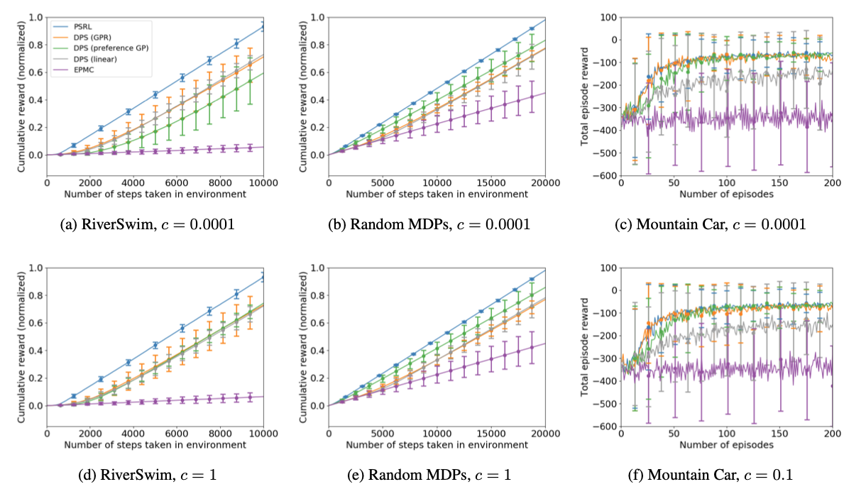
Empirical performance of DPS: Each simulated environment is shown under the two least-noisy user preference models that were evaluated. The plots show DPS with three models: Gaussian process regression (GPR), Bayesian linear regression, and a Gaussian process preference model.
Novoseller et al. (2020)
3. Dueling Posterior Sampling
Plots display the mean +/- one standard deviation over 100 runs of each algorithm tested. Overall, we see that DPS performs well and is robust to the choice of credit assignment model.
Novoseller et al. (2020)
Summary
- The dueling bandit problem is a variant of the multi-armed bandit problem where the learner receives pairwise comparisons between arms.
- Several algorithms have been proposed to solve the dueling bandit problem, such as \(\epsilon\)-greedy, UCB, and Thompson sampling.
- In the case of contextual dueling bandits, the learner receives context information along with the pairwise comparisons.
- The DPS algorithm is a preference-based reinforcement learning algorithm capable of solving contextual bandits that use Bayesian linear regression to model the utility function and Thompson sampling to select policies.
- The DPS algorithm is asymptotically optimal in terms of Bayesian regret.
Discussion and Q&A
Next Lecture:
Preferential Bayesian Optimization
![]()
Chapter 4.1: Dueling Bandits