Machine Learning from Human Preferences
Chapter 2: Choice Models (Part 2)
The ideal point model
- An embedding approach, assumes user item preference depends on distance
- Let \(x_n\) denote a latent vector representing an individual \(n\)
- Let \(v_i\) denote a latent vector representing choice (or item) \(i\) \(U_{ni} = dist(x_n, v_i) + \epsilon_{ni}\)
- Model is equivalent to choosing the “closest” item
\[
y_{ni} =
\begin{cases}
1, & \text{if } U_{ni} > U_{nj} \ \forall j \neq i \\
0, & \text{otherwise}
\end{cases}
\]
Ideal point model: the why
- Pros: Can sometimes learn preferences faster than attribute-based preference models by exploiting geometry (see refs)
- Cons:
- Embedding assumption may be strong (can make more flexible via distance function choice)
- However, have to select a distance function (usually use Euclidian distance in the embedding)
Jamieson and Nowak (2011); Tatli, Nowak, and Vinayak (2022)
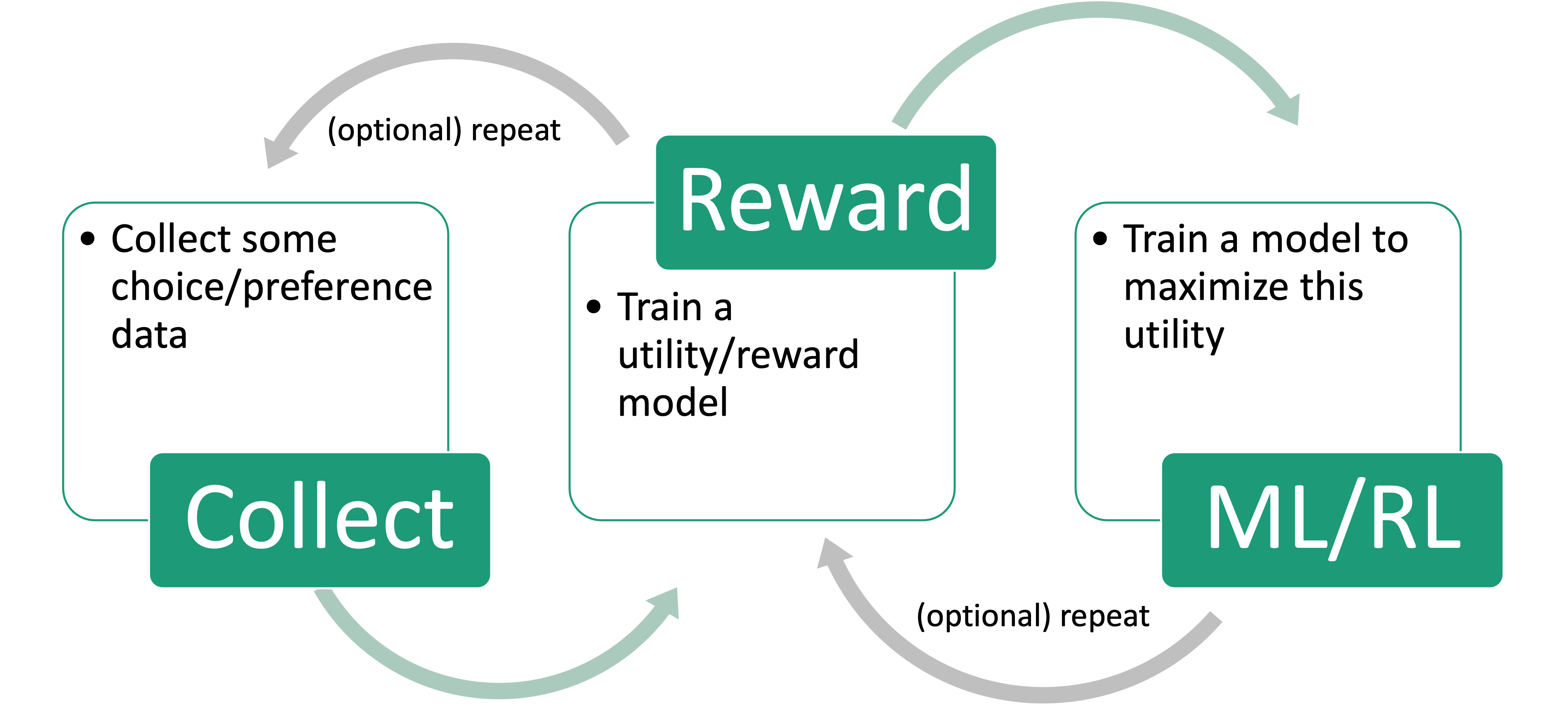
Choice models in RL (and RLHF)
![]()
Choice models in RL
Application: RL and Language
(Bradley-Terry model)
![]()
RLHF
https://openai.com/research/learning-to-summarize-with-human-feedback
Choice models in ML (recommender systems, bandits, Direct Preference Optimization)
![]()
Model in ML
Choice models in ML (recommender systems, bandits, DPO)
![]()
Model in ML
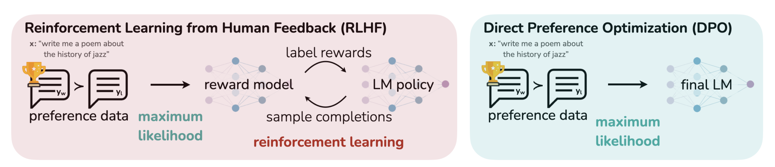
Why DPO?
![]()
DPO vs PPO
- RLHF pipeline is complex and unstable due to the reward model optimization.
- DPO is more stable and can be used to optimize the reward model directly.
Rafailov et al. (2023)
DPO: Bradley-Terry model
- Given prompt \(x\) and completions \(y_w\) and \(y_l\) the choice model gives the preference
\[
p^*(y_w > y_l | x) = \frac{\exp(r^*(x, y_w))}{\exp(r^*(x, y_w)) + \exp(r^*(x, y_l))}
\]
where \(r^*(x, y)\) is some latent reward model that we do not have access to (i.e., the human preference)
DPO: Bradley-Terry model
Luckily, we can use parameterize the reward model with some neural networks with parameters \(\phi\):
Let us start with the Reward Maximization Objective in RL: \[
\max_{\pi_\theta} \mathbb{E}_{x \sim \mathcal{D}, y \sim \pi_\theta(y|x)} [r_\phi(x, y) - \beta D_{KL}(\pi_\theta(y|x) \| \pi_{\text{ref}}(y|x))]
\]
- Where \(\pi_\theta(y|x)\) is the language model, and \(\pi_{\text{ref}}(y|x)\) is the reference model (e.g., the language model before fine-tuning)
\[
\max_{\pi_\theta} \mathbb{E}_{x \sim \mathcal{D}, y \sim \pi_\theta(y|x)} [r_\phi(x, y) - \beta D_{KL}(\pi_\theta(y|x) \| \pi_{\text{ref}}(y|x))]
\]
Recall the definition of KL divergence: \[
D_{KL}(p \| q) = \sum_{x \in \mathcal{X}} p(x) \log \frac{p(x)}{q(x)} = \mathbb{E}_{x \sim \mathcal{X}} \left[ \log \frac{p(x)}{q(x)} \right]
\]
Then we can rewrite the objective as: \[
\begin{aligned}
&\max_{\pi_\theta} \mathbb{E}_{x \sim \mathcal{D}, y \sim \pi_\theta(y|x)} \left[ r_\phi(x, y) - \beta \mathbb{E}_{y \sim \pi_\theta(y|x)} \left[\log \frac{\pi_\theta(y|x)}{\pi_{\text{ref}}(y|x)} \right] \right]\\
&=\max_{\pi_\theta} \mathbb{E}_{x \sim \mathcal{D}} \mathbb{E}_{y \sim \pi_\theta(y|x)} \left[ r_\phi(x, y) - \beta \log \frac{\pi_\theta(y|x)}{\pi_{\text{ref}}(y|x)} \right]
\end{aligned}
\]
Then, we can continue to derive the objective as: \[
\begin{aligned}
&\max_{\pi_\theta} \mathbb{E}_{x \sim \mathcal{D}} \mathbb{E}_{y \sim \pi_\theta(y|x)} \left[ r_\phi(x, y) - \beta \log \frac{\pi_\theta(y|x)}{\pi_{\text{ref}}(y|x)} \right] \\
&\propto \min_{\pi_\theta} \mathbb{E}_{x \sim \mathcal{D}} \mathbb{E}_{y \sim \pi_\theta(y|x)} \left[ \log \frac{\pi_\theta(y|x)}{\pi_{\text{ref}}(y|x)} - \frac{1}{\beta} r_\phi(x, y) \right] \text{// reverse and divide } \beta\\
&= \min_{\pi_\theta} \mathbb{E}_{x \sim \mathcal{D}} \mathbb{E}_{y \sim \pi_\theta(y|x)} \left[ \log \frac{\pi_\theta(y|x)}{\frac{1}{Z(x)} \pi_{\text{ref}}(y|x) \exp\left(\frac{1}{\beta} r_\phi(x, y)\right)} - \log Z(x) \right]
\end{aligned}
\]
\[
\text{with} \quad Z(x) = \sum_{y} \pi_{\text{ref}}(y|x) \exp\left(\frac{1}{\beta} r_\phi(x, y)\right)
\]
Because \(Z(x)\) is a constant with respect to \(\pi_\theta\), we can define: \[
\pi^*(y|x) = \frac{1}{Z(x)} \pi_{\text{ref}}(y|x) \exp\left(\frac{1}{\beta} r_\phi(x, y)\right)
\]
Then, we can rewrite the optimization problem as: \[
\min_{\pi_\theta} \mathbb{E}_{x \sim \mathcal{D}} \mathbb{E}_{y \sim \pi_\theta(y|x)} \left[ \log \frac{\pi_\theta(y|x)}{\pi^*(y|x)} - \log Z(x) \right]
\]
\[
= \min_{\pi_\theta} \mathbb{E}_{x \sim \mathcal{D}} \mathbb{E}_{y \sim \pi_\theta(y|x)} \left[ \mathbb{D}_{KL}(\pi_\theta(y|x) \| \pi^*(y|x)) - \log Z(x) \right]
\]
Thus, the optimal solution (i.e., the optimal language model) is: \[
\pi_\theta(y|x) = \pi^*(y|x) = \frac{1}{Z(x)} \pi_{\text{ref}}(y|x) \exp\left(\frac{1}{\beta} r_\phi(x, y)\right)
\]
With some algebra, we can show that the optimal reward model is: \[
\begin{aligned}
\pi_\theta(y|x) &= \frac{1}{Z(x)} \pi_{\text{ref}}(y|x) \exp\left(\frac{1}{\beta} r_\phi(x, y)\right)\\
\log \pi_\theta(y|x) &= \log \pi_{\text{ref}}(y|x) + \frac{1}{\beta} r_\phi(x, y) - \log Z(x) \text{// perform } \log(.)\\
r_\phi(x, y) &= \beta \log \frac{\pi_\theta(y|x)}{\pi_{\text{ref}}(y|x)} + \beta \log Z(x)\\
\end{aligned}
\]
Recall the Bradley-Terry model with parameterized reward model: \[
p_\phi(y_w > y_l | x) = \frac{\exp(r_\phi(x, y_w))}{\exp(r_\phi(x, y_w)) + \exp(r_\phi(x, y_l))}
\]
We also have the optimal reward model: \[
r_\phi(x, y) = \beta \log \frac{\pi_\theta(y|x)}{\pi_{\text{ref}}(y|x)} + \beta \log Z(x)
\]
Thus, we can rewrite the choice model as: \[
\begin{aligned}
p_\phi(y_w \succ y_l | x) &= \frac{1}{1 + \exp\left( \beta \log \frac{\pi_\theta(y_l | x)}{\pi_{\text{ref}}(y_l | x)} - \beta \log \frac{\pi_\theta(y_w | x)}{\pi_{\text{ref}}(y_w | x)} \right)}\\
&= \sigma\left( \beta \log \frac{\pi_\theta(y_w | x)}{\pi_{\text{ref}}(y_w | x)} - \beta \log \frac{\pi_\theta(y_l | x)}{\pi_{\text{ref}}(y_l | x)} \right)
\end{aligned}
\]
DPO: Bradley-Terry model
Recall our objective to maximize the reward model, we can rewrite the objective as maximizing the likelihood of the choice model: \[
\mathcal{L} (r_\theta, \mathcal{D}) = - \mathbb{E}_{(x, y_w, u_l) \sim \mathcal{D}} \left[ \log p_\phi(y_w \succ y_l | x) \right]
\]
Finally, we can rewrite the objective as:
\[
\begin{aligned}
\mathcal{L}_{DPO}(\pi_\theta; \pi_{\text{ref}}) &= - \mathbb{E}_{(x, y_w, u_l) \sim \mathcal{D}} \left[ \log p_\phi(y_w \succ y_l | x) \right]\\
&= -\mathbb{E}_{(x, y_w, y_l) \sim D} \left[ \log \sigma\left( \beta \log \frac{\pi_\theta(y_w | x)}{\pi_{\text{ref}}(y_w | x)} - \beta \log \frac{\pi_\theta(y_l | x)}{\pi_{\text{ref}}(y_l | x)} \right) \right]
\end{aligned}
\]
Rafailov et al. (2023)
![]()
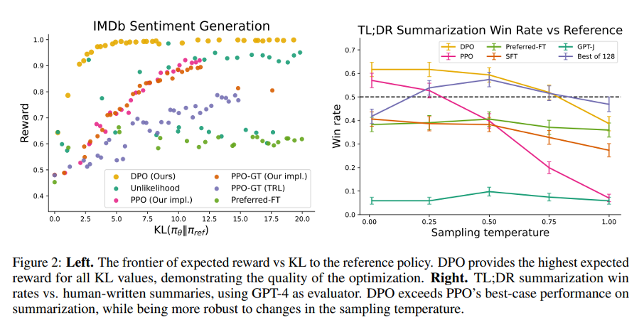
RLHF Comparison
Should your ML application use an explicit utility/reward model?
- Pro:
- Reward models can be re-used (in principle)
- Reward model can be examined to infer properties of human(s), and measure the quality of the preference model(s)
- Reward model(s) add useful inductive biases to the training pipeline
- Cons:
- The extra step of reward modeling can introduce (unnecessary?) errors
- Reward model optimization can be unstable (e.g., in RLHF, as argued by DPO)
Some criticisms of choice modeling more broadly
- Real-world choices often appear to be highly situational or context-dependent e.g., way choice is posed, emotional states, other factors not well modeled.
- Arguably what is exploited by marketing. Related to framing effects (more later).
- A partial rebuttal: In principle, can always add more context to the model.
- Many choices are intuitive rather than rational, so utility optimization models do not apply
- Please have limited attention and cognitive capability, especially for less salient choices
- Default choices are powerful, e.g., in 401K, or opt-in organ donors
Q & A
- What are some key assumptions in (discrete) choice models?
- Rationality (existence of a utility function that determines choices)
- Parametric model for utility and choice noise
- Finite set of choices, and explicit alternatives
- How does one apply discrete choice models to ML/RL applications with changing context (input)
- Model utility via generic models (e.g., deep neural networks)
- What are some criticisms of discrete choice models?
- Humans display context-dependent choices
- Humans often make intuitive (or irrational) choices
What is not covered
- Details of estimation, analysis
- Maximum likelihood is generally equivalent to standard classification/ranking
- Existing analysis (though often interesting) is mostly for linear (or simpler) utilities
- Many of the interesting theoretical questions are for active querying settings
- Beyond discrete choice models
- With equivalent alternatives (\(U_1 > U_2, U_1 \approx U_3\))
- Continuous “choices” e.g., pricing, demand/supply
- Dynamic discrete choice (for time varying choices) \(\approx\) RL
- Experimental design for “stated preferences”
- How to design a survey to measure alternatives, conjoint analysis
- Active querying (future discussion)
Summary
- Today: Overview of discrete choice models
- Basics of discrete choice and rationality assumptions
- Benefits and criticisms of discrete choice
- Some special cases and applications of discrete choice models to ML
- Next Lecture: Student discussion on Human Decision Making and Choice Models