Machine Learning from Human Preferences

Chapter 2: Choice Models (Part 1)

Overview

• Tools to predict the choice behavior of a group of decision-makers in a specific choice context.
• Thurstone research into food preferences in the 1920s.

Application: Marketing

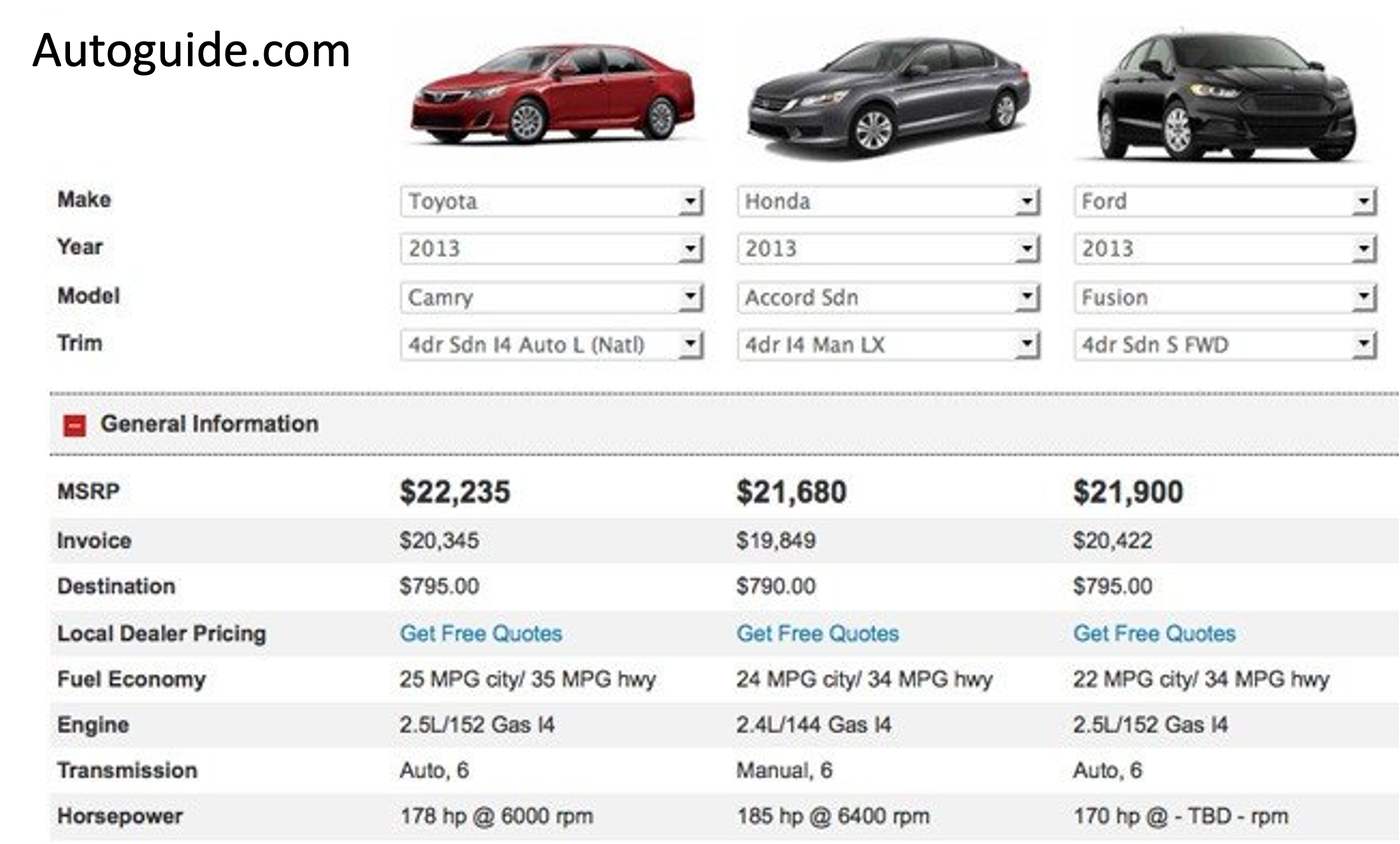
• Marketing: Predict demand for new products that are potentially expensive to produce
• What features affect a car purchase?

Application: Economics

• Microeconomics: Random Utility Theory (1970s) (McFadden: 2000 Nobel prize for the theoretical basis for discrete choice)
• Energy Economics:

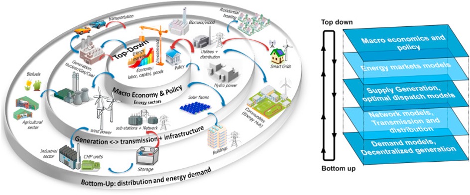
Del Granado et al. (2018)

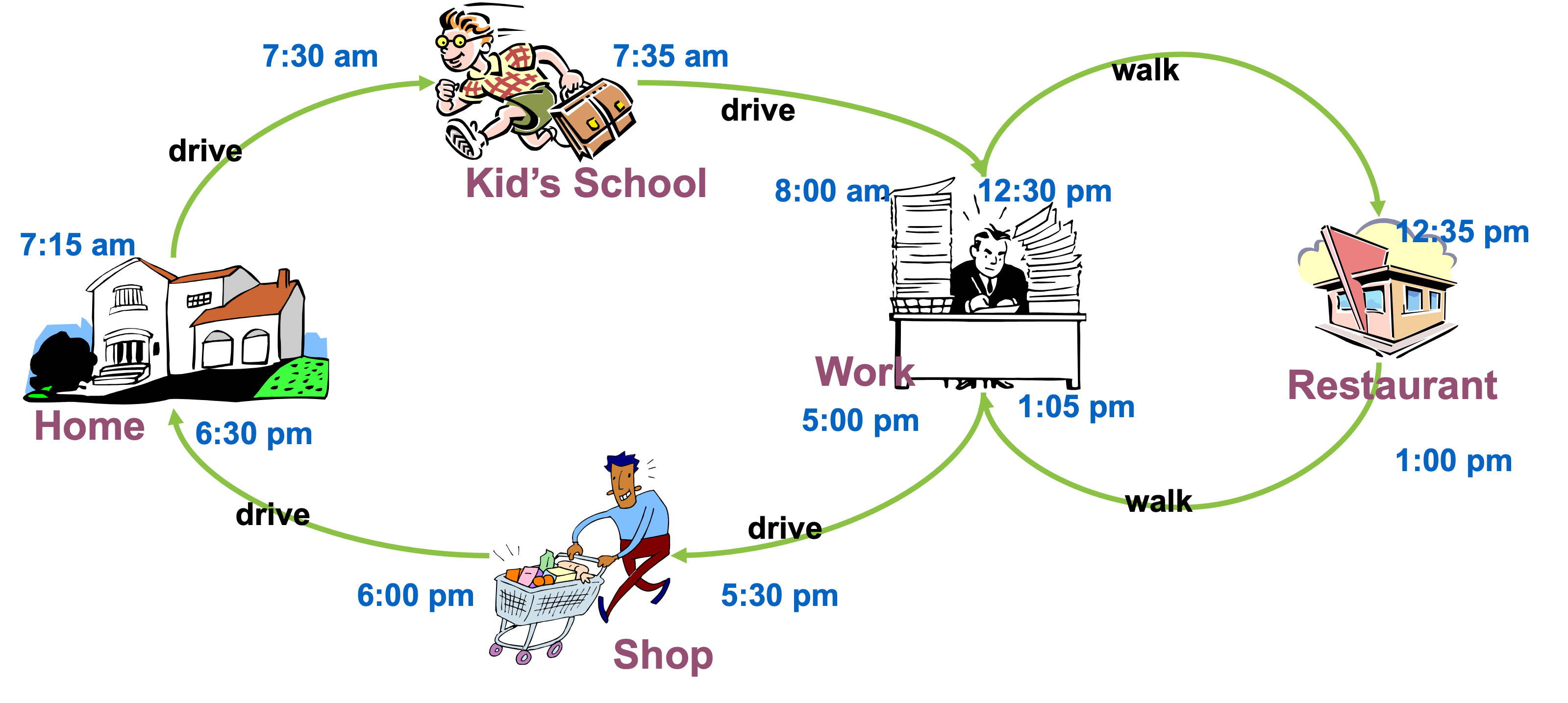
Example: Daily activity-travel pattern of an individual. Source: Chandra Bhat, “General introduction to choice modeling”

Application: Transportation

• Transportation: Predict usage of transportation resources, e.g., used by McFadden to predict the demand for the Bay Area Rapid Transit (BART) before it was built
• How pricing affects route choice
• How much is a driver willing to pay

Image source: supplychain247.com

Application: Psychology

• Psychology: Duncan Luce and Anthony Marley (Luce 1959. Conditional logit analysis of qualitative choice behavior)

Application: RL and Language

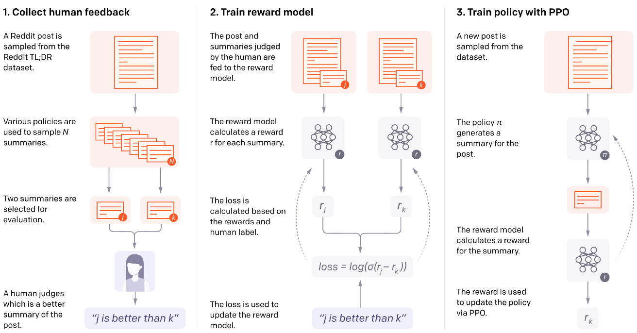
https://openai.com/research/learning-to-summarize-with-human-feedback

Motivations

• Human preferences are often gathered by asking for choices across alternatives
• Basic choice models are the workhorse for ML from preferences (Bradley-Terry, Plackett Luce)
• Our discussion will highlight some of the key assumptions, e.g., utility and rationality
• We will cover models originally built for discrete/finite choices, which have been extended to ML applications (conditional choices)

Discrete Options

• Models designed to capture decision-process of individuals
• True utility is not observable, but perhaps can measure via preferences over choices
• Main assumption: utility (benefit, or value) that an individual derives from item A over item B is a function of the frequency that they choose item A over item B in repeated choices.
• Useful Note: “Utility” in choice models <=> “Reward” in RL

Discrete Options

• Choices are collectively exhaustive, mutually exclusive, and finite

\[ y_{ni} = \begin{cases} 1, & \text{if } U_{ni} > U_{nj} \ \forall j \neq i \\ 0, & \text{otherwise} \end{cases} \]

\[ U_{ni} = H_{ni}(z_{ni}) \]

• \(z_{n,i}\) are variables describing the individual attributes and the alternative choices
• \(H_{ni}(z_{ni})\) is a stochastic function, e.g., linear: \(H_{ni}(z_{ni}) = \beta z_{ni} + \epsilon_{ni}\), where \(\epsilon_{ni}\) are unobserved individual factors

Implications

• Only the utility differences matter \[ \begin{aligned} P_{ni} &= Pr(y_{ni} = 1) \\ &= Pr(U_{ni} > U_{nj}, \forall j \neq i) \\ \end{aligned} \]
• Note that utility here is scale-free
  • It may be invariant to monotonic transformations
  • The scale works within a single context, but requires normalization for comparing across datasets.
  • A common approach is to normalize scale by standardizing the variance.

Example: Binary Choice

Binary choice with individual attributes

• Benefit of action depends on \(s_n\) = individual characteristics \[ \begin{cases} U_n = \beta s_n + \epsilon_n \\ y_n = \begin{cases} 1 & U_n > 0 \\ 0 & U_n \leq 0 \end{cases} \end{cases} \] \[ \quad \Rightarrow \quad P_{n1} = \frac{1}{1 + \exp(-\beta s_n)} \]
• \(\epsilon \sim\) Logistic

Example: Binary Choice

Binary choice with individual attributes

• Replacing \(\epsilon \sim\) Standard Normal gives the probit model \[P_{n1} = \Phi(\beta s_n)\]
• Where \(\Phi(.)\) is the normal CDF

Example: Bradley-Terry Model

Utility is linear function of variables that vary over alternatives

• The utility of each alternative depends on the attributes of the alternatives (which may include individual attributes)
• Unobserved terms are assumed to have an extreme value distribution

Example: Bradley-Terry Model

Utility is linear function of variables that vary over alternatives

\[ \begin{cases} U_{n1} = \beta z_{n1} + \epsilon_{n1} \\ U_{n2} = \beta z_{n2} + \epsilon_{n2} \\ \epsilon_{n1}, \epsilon_{n2} \sim \text{iid extreme value} \end{cases} \] \[ \Rightarrow \quad P_{n1} = \frac{\exp(\beta z_{n1})}{\exp(\beta z_{n1}) + \exp(\beta z_{n2})} = \frac{1}{1 + \exp(-\beta (z_{n1} - z_{n2}))} \]

• We can replace noise with Standard Normal: \(P_{n1} = \Phi(\beta (z_{n1} - z_{n2}))\)

Example: Multiple Alternatives

Utility for each alternative depends on attributes of that alternative

• Unobserved terms are assumed to have an extreme value distribution
• With \(J\) alternatives \[ \begin{cases} U_{ni} = \beta z_{ni} + \epsilon_{ni} \\ \epsilon_{ni} \sim \text{iid extreme value} \end{cases} \quad \Rightarrow \quad P_{ni} = \frac{\exp(\beta z_{ni})}{\sum_{j=1}^{J} \exp(\beta z_{nj})} \]

Example: Multiple Alternatives

Utility for each alternative depends on attributes of that alternative

• Compare to standard model for multiclass classification (multiclass logistic)
• Can also replace noise model with Gaussians

Alternative Correlations

Capturing correlations across alternatives

• All the prior models use the logistic model which does not capture correlations in noise.
• This can be fixed using a joint distribution over the noise e.g., \[ \begin{cases} U_{ni} = \beta z_{ni} + \epsilon_{ni} \\ \epsilon_n \equiv (\epsilon_{n1}, \cdots, \epsilon_{nJ}) \sim N(0, \Omega) \end{cases} \]

Estimation

• Linear case: maximum likelihood estimators (logistic and probit regression)
• More complex function classes: use standard ML fitting tools for (regularized) maximum likelihood, e.g., stochastic gradient descent (SGD)
• Standard tradeoffs, e.g., bias-variance tradeoff
  • More complex models generally require more data
  • Most ML applications pool data across individuals whose differences may matter (future discussion)

Measuring Ordered Preferences

• Example: On a 1-5 scale (1: disagree completely, 5: agree completely) how much do you agree with the statement “I am enjoying this class so far”?
• To analyze the data, we use ordinal regression, \(U_n = H_n(z_n)\), for some real parameters \(a, b, c, d\) \[ y_n = \begin{cases} 1, & \text{if } U_n < a \\ 2, & \text{if } a < U_n < b \\ 3, & \text{if } b < U_n < c \\ 4, & \text{if } c < U_n < d \\ 5, & \text{if } U_n > d \end{cases} \]

Ordered Logit

• For linear utility: \(U_n = \beta z_n + \epsilon\), \(\epsilon \sim\) Logistic

\(Pr(\text{choosing 1}) = Pr(U_n < a) = Pr(\epsilon < a - \beta z_n) = \frac{1}{1 + \exp(-(a - \beta z_n))}\)

\(\begin{aligned} Pr(\text{choosing 2}) &= Pr(a < U_n < b) = Pr(a - \beta z_n < \epsilon < b - \beta z_n) \\ &= \frac{1}{1 + \exp(-(b - \beta z_n))} - \frac{1}{1 + \exp(-(a - \beta z_n))} \end{aligned}\)

\(...\)

\(Pr(\text{choosing 5}) = Pr(U_n > d) = Pr(\epsilon > d - \beta z_n) = 1 - \frac{1}{1 + \exp(-(d - \beta z_n))}\)

• We can also replace the Logistic with Gaussian for ordered probit regression

Plackett-Luce Model

• PL model ranks items based on the sequence of choices.
• The probability of choice ranking 1, 2, …, J is calculated:

\[Pr(\text{ranking } 1, 2, \dots, J) = \frac{\exp(\beta z_1)}{\sum_{j=1}^{J} \exp(\beta z_{nj})} \cdot \frac{\exp(\beta z_2)}{\sum_{j=2}^{J} \exp(\beta z_{nj})} \cdots \frac{\exp(\beta z_{J-1})}{\sum_{j=J-1}^{J} \exp(\beta z_{nj})}\]

• This model is commonly used in biomedical literature.
• It is also known as rank ordered logit (econometrics ~1980s), or exploded logit model.
• All mentioned extensions also apply to this model (nonlinear utility, correlated noise, etc.).

Modeling and Estimation Summary

• Choose the utility model, i.e., how the attributes and alternatives define the utility e.g., linear function of attributes with logistic noise
• Choose the response/observation model, e.g., binary, multiple choice, ordered choice.
• Fit the model using (regularized) maximum likelihood

Revealed vs Stated Preference

• Revealed preference: We generally use offline observational real choices to estimate item value.
• Stated Preference: We generally use online observational choices under experimental conditions.
• Revealed preference is considered a ‘real’ choice that can be more accurate, whereas participants in simulated situations may not respond well to hypotheticals, though observed data might not cover the space like experiments can.

Exercise: Choice Model for Class

“Should you take CS 329H or not?”

“Should you take CS 329H or CS 221 or CS 229?”

• What attributes/features should be measured about the class?
• What utility model would be appropriate?
• What observation/response model should be used?
• Should revealed preference (observed choices) or stated preference (hypothetical) be employed?

Exercise: Choice Model for Language

• What utility model would be appropriate? What attributes/features should be measured about the class?
• What observation/response model should be used?
• Should revealed preference (observed choices) or stated preference (hypothetical) be employed?
• Who should you query for the evaluation? Should you use individual or pooled responses? Why or why not?
• What are some pros/cons of your design?

References

• Train (1986)
• McFadden and Train (2000)
• Luce et al. (1959)
• Additional:
  • Ben-Akiva and Lerman (1985)
  • Park, Simar, and Zelenyuk (2017)
  • Rafailov et al. (2023)

Ben-Akiva, Moshe E., and Steven R. Lerman. 1985. Discrete Choice Analysis: Theory and Application to Travel Demand. Transportation Studies. Cambridge, MA: MIT Press.

Del Granado, Pedro Crespo, Gustav Resch, Franziska Holber, Marijke Welisch, et al. 2018. “Modelling the Energy Transition: A Nexus of Energy System and Economic Models.” Energy Strategy Reviews 20: 229–35.

Luce, R Duncan et al. 1959. Individual Choice Behavior. Vol. 4. Wiley New York.

McFadden, Daniel, and Kenneth Train. 2000. “Mixed MNL Models for Discrete Response.” Journal of Applied Econometrics 15 (5): 447–70.

Park, Byeong U, Leopold Simar, and Valentin Zelenyuk. 2017. “Nonparametric Estimation of Dynamic Discrete Choice Models for Time Series Data.” Computational Statistics & Data Analysis 108: 97–120. https://doi.org/10.1016/j.csda.2016.10.024.

Rafailov, Rafael, Archit Sharma, Eric Mitchell, Stefano Ermon, Christopher D. Manning, and Chelsea Finn. 2023. “Direct Preference Optimization: Your Language Model Is Secretly a Reward Model.” https://arxiv.org/abs/2305.18290.

Train, Kenneth. 1986. Qualitative Choice Analysis: Theory, Econometrics, and an Application to Automobile Demand. MIT Press.